← return to practice.dsc40a.com
This page contains all problems about Summary Statistics and the Constant Model.
Let \vec{y}_1, \vec{y}_2, \dotsc, \vec{y}_n \in\mathbb{R}^2 be a collection of two-dimensional vectors and let \overline{y} = \frac{1}{n}\sum_{i=1}^n \vec{y}_i. Suppose we wish to model the \vec{y}_i’s using a single vector of the form c\vec{z} where \vec{z} = \begin{bmatrix} -1 & 1 \end{bmatrix}^T and c\in\mathbb{R} is a real number (to be determined).
Suppose we use the loss function L_{\mathrm{sq}}(\vec{y}_i, c) = |\vec{y}_i^{(1)} + c|^2 + |\vec{y}_i^{(2)} - c|^2. Write down the empirical risk function R_{\mathrm{sq}}(\{\vec{y}_i\}_{i=1}^n, c).
R_{\mathrm{sq}}(\{\vec{y}_i\}_{i=1}^n, c) = \frac{1}{n}\sum_{i=1}^n (|\vec{y}_i^{(1)} + c|^2 + |\vec{y}_i^{(2)} - c|^2).
Recall risk follows the formula R_{L(h)}(h) = \frac{1}{n} \sum_{i=1}^n L(h). All we have to do is put the loss function in a summation and divide it by n. It is important to put parenthesis around the loss function.
The average score on this problem was 71%.
Show that c^\ast = \frac{1}{2}\vec{z}^T \overline{y} is the only critical point for the empirical risk function R_{\mathrm{sq}}(\{\vec{y}_i\}_{i=1}^n, c) you found in part (a).
\begin{align*} \frac{\partial}{\partial c} R_{\mathrm{sq}}((\vec{y}_i), c) &= \frac{\partial}{\partial c} \frac{1}{n}\sum_{i=1}^n (|\vec{y}_i^{(1)} + c|^2 + |\vec{y}_i^{(2)} - c|^2)\\ &= \frac{1}{n}\sum_{i=1}^n \left( 2(\vec{y}_i^{(1)} + c)- 2(\vec{y}_i^{(2)} - c)\right)\\ &= 4c - \frac{2}{n}\sum_{i=1}^n \vec z^T \vec{y}_i\\ &=4c - 2\vec{z}^T \overline{y}. \end{align*} Therefore, the one critical point occurs when c = \frac{1}{2}\vec{z}^T \overline{y}.
The average score on this problem was 63%.
Given the dataset: \vec{y_1}=\begin{bmatrix} 1 \\ - 2 \end{bmatrix} \quad \vec{y_2}=\begin{bmatrix} -3 \\ 4 \end{bmatrix} \quad \vec{y_3}=\begin{bmatrix} 2 \\ - 2 \end{bmatrix} what is R_{\mathrm{sq}}(\{\vec{y}_1, \vec{y}_2, \vec{y}_3\}, c^\ast)?
\vec y = \begin{bmatrix} 0\\ 0 \end{bmatrix}
c^*=\frac{1}{2}\vec{z}^T \overline{y} = 0
\begin{align*} R_{\mathrm{sq}}((\vec{y}_i), c) & = \frac{1}{n}\sum_{i=1}^n \left(|\vec{y}_i^{(1)} - c|^2 + |\vec{y}_i^{(2)} - c|^2\right) \\ & = \frac{1}{3} \left( (1^2+2^2) + (3^2+4^2) + (2^2+2^2) \right) = \frac{38}{3} \end{align*}
The average score on this problem was 57%.
Assume you have a dataset \vec{x}_1, \vec{x}_2, \dotsc, \vec{x}_n\in\mathbb{R}^{d} of d-dimensional vectors for n individuals, and that each has a scalar response value y_1,\dotsc, y_n. You then fit a multiple linear regression prediction rule H_1(\vec{x}) = \vec{w}^T\text{Aug}(\vec{x}), with optimal parameters \vec{w}^* whose MSE is c_1.
Due to privacy reasons it turns out you are unable to use the feature x^{(d)}, so you need to find a way to modify your model so that it does not incorporate this feature. Your friend Minnie suggests using the parameters of the prediction rule you learned already and simply setting w_d=0: H_2(\vec{x}) = \begin{bmatrix} w_0^* & w_1^* & \ldots & w_{d-1}^* & 0 \end{bmatrix}^T \text{Aug}(\vec{x}). Denote the MSE of the model H_2(\vec{x}) by c_2.
Meanwhile, your friend Maxine recommends fitting a new prediction rule H_3 to the data with only the first d-1 features, with MSE c_3.
Order the three errors c_1, c_2, c_3 from least to greatest. Explain your solution. (Use < if the error is strictly smaller, = if the errors are equal or \leq if the errors may be equal.)
c_1 \leq c_3 \leq c_2.
The prediction rule H_1 uses an additional feature compared to H_3. The MSE cannot increase by adding a feature (HW4), therefore c_1 \leq c_3.
The MSE c_3 is as small as it can possibly be when using d-1 features. If we were to pick other coefficients – whatever they may be – the MSE cannot be smaller. So if we picked the coefficients (w^*_0, w^*_1, \ldots, w^*_{d-1}), note that setting w_d=0 in H_2 is the same as setting a prediction rule with d-1 features and the first d parameters of w^*. Since this prediction rule is using d-1 features, the MSE c_2 of this model cannot be smaller than c_3.
The average score on this problem was 65%.
You are able to add 5 additional individuals to your datasets, so that now you have n+5 individuals. You fit a new prediction rule to the data whose MSE is c_4. Can c_4< c_1? Explain.
In the case you add 5 individuals that exactly match the prediction rule, their added squared errors are all zero and therefore the mean squared error is smaller c_4 = \frac{n c_1}{n+5}.;
The average score on this problem was 41%.
Source: Summer Session 2 2024 Final, Problem 1a-g
Consider the dataset x_1 = 1, x_2 = 2, x_3 = 3, x_4 = 4, x_5 = 5.
Which single element of the dataset would you change, and to what value, to make h^* = 4 the single minimizing value for the following loss function and corresponding empirical risk? Bubble in your choice of x_i, if possible, and provide the new value of that x_i. If no such x_i is possible, bubble in “Not possible" and explain why. L(y_i, h) = \begin{cases} 0 & y_i = h \\ 1 & y_i \neq h \end{cases}
x_1
x_2
x_3
x_4
x_5
Not possible
Include an explanation.
x_1 = 4 or x_2 = 4 or x_3 = 4 or x_5 = 4
Recall from lecture 0-1 loss L(y_i, h) = \begin{cases} 0 & y_i = h \\ 1 & y_i \neq h \end{cases} is minimized by the mode. This means we want to maximize the number of matches between h and y_i. If h^* = 4 then we want to change values that are not equal to 4 into 4. This means any answer that is not x_4 can be changed to equal 4 and it is possible.
The average score on this problem was 64%.
Suppose we must modify x_5. What should the new value of x_5 be to make h^* = 6 for the following loss function and corresponding empirical risk?
L(y_i, h) = (y_i - h)^2
x_5 should be modified to 20
We know that L(y_i, h) = (y_i - h)^2 is minimized by the mean. This means h^* = \frac{1}{n} \sum_{i = 1}^n x_i.
We can make the equation h^* =6 by writing 6 = \frac{1 + 2 + 3 + 4 + x_5'}{5}. From here we simply solve for x_5'.
\begin{align*} 6 &= \frac{1 + 2 + 3 + 4 + x_5'}{5}\\ 30 &= 1 + 2 + 3 + 4 + x_5'\\ 30 &= 10 + x_5 \\ 20 &= x_5 \end{align*}
Here we can see that x_5 should be changed to 20.
The average score on this problem was 83%.
Suppose we must modify x_1. What should the new value of x_1 be to make h^* = 6 for the following loss function and corresponding empirical risk?
L(y_i, h) = (y_i - h)^2
x_1 should be modified to 16
Once again we know that L(y_i, h) = (y_i - h)^2 is minimized by the mean. This means h^* = \frac{1}{n} \sum_{i = 1}^n x_i.
We can make the equation h^* =6 by writing 6 = \frac{x_1' + 2 + 3 + 4 + 5}{5}. From here we simply solve for x_1'.
\begin{align*} 6 &= \frac{x_1' + 2 + 3 + 4 + 5}{5}\\ 30 &= x_1 + 2 + 3 + 4 + 5\\ 30 &= x_1 + 14 \\ 16 &= x_1 \end{align*}
Here we can see that x_1 should be changed to 16.
The average score on this problem was 83%.
Consider the dataset x_1 = 1, x_2 = 2, x_3 = 3, x_4 = 4, x_5 = 5.
Which single element of the dataset would you change, and to what value, to make h^* = 4 for the following loss function and corresponding empirical risk? Bubble in your choice of x_i, if possible, and provide the new value of that x_i in the box below. If no such x_i is possible, bubble in “Not possible" and explain why in the box below. L(y_i, h) = |y_i - h|
x_1
x_2
x_3
x_4
x_5
Not possible
Include an explanation.
x_3 = 4
This is absolute loss and is minimized by the median. This means we need to turn whatever the current median is into 4.
When we look at the dataset (x_1 = 1, x_2 = 2, x_3 = 3, x_4 = 4, x_5 = 5) we can see the current median is x_3 = 3. This means all we need to do is change the x_3 to 4.
The average score on this problem was 89%.
Which single element of the dataset would you change, and to what value, to make h^* = 5 for the following loss function and corresponding empirical risk? Bubble in your choice of x_i, if possible, and provide the new value of that x_i in the box below. If no such x_i is possible, bubble in “Not possible" and explain why in the box below. L(y_i, h) = |y_i - h|
x_1
x_2
x_3
x_4
x_5
Not possible
Include an explanation.
Not possible
This is absolute loss and is minimized by the median. This means we need to turn whatever the current median is into 4.
When we look at the dataset (x_1 = 1, x_2 = 2, x_3 = 3, x_4 = 4, x_5 = 5) we can see the current median is x_3 = 3. However, if we change x_3 = 5 then the dataset would look like: x_1 = 1, x_2 = 2, x_4 = 4, x_3 = 5, x_5 = 5, which would make the median equal to 4. There is no way to make the median 5 by only changing a single value.
The average score on this problem was 92%.
Suppose we delete x_2, so the dataset is x_1 = 1, x_3=3, x_4=4, x_5=5. What is the new value of h^* for following loss function and corresponding empirical risk? L(y_i, h) = (y_i - h)^2
The mean of the dataset: \frac{13}{4}
Once again we know that L(y_i, h) = (y_i - h)^2 is minimized by the mean. This means h^* = \frac{1}{n} \sum_{i = 1}^n x_i.
If we delete x_2 this means our equation becomes \frac{1 + 3 + 4 + 5}{4} = \frac{13}{4}.
The average score on this problem was 88%.
Suppose we delete x_3, so the dataset is x_1 = 1, x_2=2, x_4=4, x_5=5. Which of the following values of h^* minimize the following loss function and corresponding empirical risk? L(y_i, h) = |y_i - h|
1
1.5
2
2.5
3
3.5
4
4.5
5
2, 2.5, 3, 3.5, 4
Once again, recall L(y_i, h) = |y_i - h| is minimized by the median. The new dataset is even and has a median between 2 and 4, which means any answer in-between (and including) these values should be selected.
The average score on this problem was 87%.
Source: Summer Session 2 2024 Final, Problem 2a-e
Consider a dataset of 4 values, y_1 < y_2 < y_3 < y_4, with a mean of 6.
Let Y_\text{abs}(h) = \frac{1}{4} \sum_{i = 1}^4 |y_i - h| represent the mean absolute error of a constant prediction h on this dataset of 4 values.
Similarly, consider another dataset of 3 values, x_1 < x_2 < x_3, that also has a mean of 6.
Let X_\text{abs}(h) = \frac{1}{3} \sum_{i = 1}^3 |x_i - h| represent the mean absolute error of a constant prediction h on this dataset of 3 values.
Suppose that x_1 < y_1, y_4 < x_2, and that T_\text{abs}(h) represents the mean absolute error of a constant prediction h on the combined dataset of 7 values, x_1, y_1, ..., y_4, x_2, x_3. We denote these 7 values as \{ z_1, z_2, z_3, z_4, z_5, z_6, z_7 \}.
What value of h minimizes the following empirical risk function? Z(h) = \frac{1}{7} \sum_{i = 1}^7 (h - z_i)
-\infty
0
6
y_3
Any value between y_3 and y_4
Z(h) = \frac{1}{7} \sum_{i = 1}^7 (h - z_i) is minimized when h is as small as possible. If h is smaller than z_i then it will make a negative risk! This means the smaller h is the smaller the difference will be!
When looking at our answers available the smallest risk would be h^* = -\infty.
The average score on this problem was 16%.
What value of h minimizes mean absolute error, T_\text{abs}(h)?
-\infty
0
6
y_3
Any value between y_3 and y_4
\infty
y_3, the median of the dataset.
Recall h^* for T_\text{abs}(h) is the median of the dataset!
Our dataset is: x_1, y_1, y_2, y_3, y_4, x_2, x_3. Our median is y_3, which means h^* = y_3.
The average score on this problem was 77%.
Suppose the slope of T_\text{abs}(h) is -\frac{1}{7} at some h_p. Hint: think about what values of h could have this slope.
Suppose the dataset is now modified by moving the \{x_i\} such that
y_1 < y_2 < y_3 < y_4 < x_1 <
x_2 < x_3. What would the slope of T_\text{abs}(h) be at the point whose
x-value is h_p, given this assumption?
-\frac{3}{7}
Slope of T_{abs}(h) is equal to \frac{1}{7} * \text{(number of points to the left of h - number of points to the right of h)}. If the slope of T_{abs}(h) was originally -\frac{1}{7}, there must have been four points to the right of h and 3 points to the left of h, meaning y_2<h<y_3. It follows that in the modified dataset there are 5 points to the right of h and 2 points to the left of h, meaning the slope of T_{abs}(h) must be -\frac{3}{7}
The average score on this problem was 44%.
The following information is repeated from the previous page, for your convenience.
Consider a dataset of 4 values, y_1 < y_2 < y_3 < y_4, with a mean of 6. Let Y_\text{abs}(h) = \frac{1}{4} \sum_{i = 1}^4 |y_i - h| represent the mean absolute error of a constant prediction h on this dataset of 4 values.
Similarly, consider another dataset of 3 values, x_1 < x_2 < x_3, that also has a mean of 6. Let X_\text{abs}(h) = \frac{1}{3} \sum_{i = 1}^3 |x_i - h| represent the mean absolute error of a constant prediction h on this dataset of 3 values.
Suppose that x_1 < y_1, y_4 < x_2, and that T_\text{abs}(h) represents the mean absolute error of a constant prediction h on the combined dataset of 7 values, x_1, y_1, ..., y_4, x_2, x_3. We denote these 7 values as \{ z_1, z_2, z_3, z_4, z_5, z_6, z_7 \}.
Suppose the slope of T_\text{abs}(h) is -\frac{1}{7} at some h_p. Hint: think about what values of h could have this slope.
Suppose the dataset is now modified by repeating each value y_i such that it now contains x_1, y_1, y_1, y_2, y_2, y_3, y_3, y_4, y_4, in ascending order; the ordering of the points is the same as the beginning of this question. What would the slope of T_\text{abs}(h) be at the point whose x-value is h_p, given this assumption?
There are two answers based on if you believed x_2 and x_3 was still in the dataset.
Recall the slope of T_{abs}(h) is equal to \frac{1}{7} * \text{(number of points to the left of h - number of points to the right of h)}.
Correct case 1: assumes that x_2 and x_3 are still in the dataset and finds the answer to be -\frac{1}{11}
Correct case 2: does not assume that x_2 and x_3 are still in the dataset and finds the answer to be \frac{1}{9}
The average score on this problem was 31%.
At the point whose x-value is h_{p}, select the option below that correctly describes the relationship between the slopes of Y_\text{abs}(h), X_\text{abs}(h), and T_\text{abs}(h), respectively.
Hint: We already know the slope of T_\text{abs}(h) at h_p.
\text{slope of }Y_\text{abs}(h) < \text{slope of } T_\text{abs}(h) < \text{slope of } X_\text{abs}(h)
\text{slope of }Y_\text{abs}(h) < \text{slope of } X_\text{abs}(h) < \text{slope of } T_\text{abs}(h)
\text{slope of }T_\text{abs}(h) < \text{slope of } X_\text{abs}(h) < \text{slope of } Y_\text{abs}(h)
\text{slope of }T_\text{abs}(h) < \text{slope of } Y_\text{abs}(h) < \text{slope of } X_\text{abs}(h)
\text{slope of }X_\text{abs}(h) < \text{slope of } T_\text{abs}(h) < \text{slope of } Y_\text{abs}(h)
\text{slope of }X_\text{abs}(h) < \text{slope of } Y_\text{abs}(h) < \text{slope of } T_\text{abs}(h)
Slope of X_{abs}(h) < slope of T_{abs}(h) < slope of Y_{abs}(h)
There is a key insight to make here: the slope of the mean absolute error is influenced by the distribution of points above and below h.
T_{abs}(h) represents the combined dataset (both the x’s and the y’s), so the slope reflects the overall balance between the two datasets. This means the distribution of points above and below h will be smoothed out. As a result the slope will be the least steep.
You can also think of it as: x_1, y_1, y_2, h_p, y_3, y_4, x_2, x_3. The slope of T_{abs}(h) is -\frac{1}{7}.
Y_{abs}(h) represents only the y’s. There are 4 y values and we know these points are closer together than the x values. Because the y values are more concentrated the slope will be larger! (Recall that the mean for these 4 points is 6).
You can also think of it as: y_1, y_2, h_p, y_3, y_4. The slope of Y_{abs}(h) is 0.
X_{abs}(h)represents only the x’s. There are 3 x values and we know these points are farther apart than the y values. Because the x values are more spread out the slope will be smaller! (Recall that the mean for these 3 points is 6).
You can also think of it as: x_1, h_p, x_2, x_3. The slope of X_{abs}(h) is -\frac{1}{3}.
The average score on this problem was 38%.
Source: Summer Session 2 2024 Midterm, Problem 1a-d
Consider a dataset of n values, y_1, y_2, \dots, y_n, all of which are non-negative. We are interested in fitting a constant model, H(x) = h, to the data using the ``Jack” loss function, defined as:
L_{\text{Jack}}(y_i, h) = \begin{cases} \alpha \cdot (y_i - h)^2 & \text{if } y_i \geq h, \\ \beta \cdot |y_i - h|^3 & \text{if } y_i < h, \end{cases}
where \alpha and \beta are positive constants that weight the squared and cubic loss components differently depending on whether the prediction h underestimates or overestimates the true value y_i.
Find \frac{d L_\text{Jack}}{d h}, the derivative of the Jack loss function with respect to h. Show your work, and put a \boxed{\text{box}} around your final answer.
\frac{L_{\text{Jack}}}{\partial h} = \begin{cases} -2 \alpha(y_i - h) & \text{if } y_i \geq h, \\ 3 \beta |h - y_i|^2 & \text{if } y_i < h, \end{cases}
Looking at the loss function (displayed again for your convenience), we can start by taking the derivative of the first case, when y_i \geq h:
L_{\text{Jack}}(y_i, h) = \begin{cases} \alpha \cdot (y_i - h)^2 & \text{if } y_i \geq h, \\ \beta \cdot |y_i - h|^3 & \text{if } y_i < h, \end{cases}
To find the derivative of the first case we will use chain rule. Chain rule states F'(h) = f'(g(h)) \times g'(h). We start with \frac{\partial}{\partial h} \alpha(y_i - h)^2 and treat f(h) = h^2 and g(h) = (y_i - h). We can easily find f'(h) = 2h and g'(h) = -1. When combining all of these parts we get
\frac{\partial}{\partial h} \alpha(y_i - h)^2 \rightarrow -2 \alpha(y_i - h)
We can now look at the second case, when y_i < h. Once again we will use the chain rule. We start with \frac{\partial}{\partial h} \beta \cdot |y_i - h|^3 and treat f(h) = h^3 and g(h) = |y_i - h|. We can easily find f'(h) = 3h, but g'(h) is a bit trickier.
This requires you to know when h = y_i the line is undefined. This means we have a piecewise function.
g'(h) = \begin{cases} -3 \beta & \text{if } y_i > h, \\ \text{undefined} & \text{if } y_i = h\\ 3 \beta & \text{if } y_i < h, \end{cases}
Since we only care about when y_i < h we can replace g'(h) with 1! This means we have
\frac{\partial}{\partial h} \beta \cdot |y_i - h|^3 \rightarrow 3 \beta |h - y_i|^2
\boxed{\frac{L_{\text{Jack}}}{\partial h} = \begin{cases} -2 \alpha(y_i - h) & \text{if } y_i \geq h, \\ 3 \beta |h - y_i|^2 & \text{if } y_i < h, \end{cases}}
The average score on this problem was 66%.
Prove that for the constant prediction h^* minimizing empirical risk for the Jack loss function, the following quantities sum to 0:
Hint: You do not need to solve for the optimal value of h^*. Instead, walk through the general process of minimizing a risk function, and think about the equations you come across.
Once again, recall Jack loss:
L_{\text{Jack}}(y_i, h) = \begin{cases} \alpha \cdot (y_i - h)^2 & \text{if } y_i \geq h, \\ \beta \cdot |y_i - h|^3 & \text{if } y_i < h, \end{cases}
We can rewrite this to say:
L_{\text{Jack}}(y_i, h) = \alpha \cdot (y_i - h)^2 + \beta \cdot |y_i - h|^3
From here we can now set up the equation for risk. We are told in the hint to go through the motions of finding h^* without doing all of the calculations. Recall risk follows the equation: R_{\text{f(x)}} = \frac{1}{n} \sum_{i = 1}^{n} f(x). Once we have this equation we take the derivative and set it equal to zero to solve for h^*.
\begin{align*} R_{L_{\text{Jack}}} &= \frac{1}{n} \sum_{i = 1}^{n} \alpha \cdot (y_i - h)^2 + \beta \cdot |y_i - h|^3\\ &=\frac{1}{n} (\sum_{\text{if }y_i \geq h} \alpha \cdot (y_i - h)^2 + \sum_{\text{if }y_i < h} \beta \cdot |y_i - h|^3)\\ &\text{To get the derivative use part a!}\\ &= \frac{1}{n} (\sum_{\text{if }y_i \geq h} -2 \alpha(y_i - h) + \sum_{\text{if }y_i < h} 3 \beta |h - y_i|^2)\\ \end{align*}
From here we can set R_{L_{\text{Jack}}} to zero.
\begin{align*} 0 &= R_{L_{\text{Jack}}} \\ 0 &= \frac{1}{n} (\sum_{\text{if }y_i \geq h} -2 \alpha(y_i - h) + \sum_{\text{if }y_i < h} 3 \beta |h - y_i|^2) \\ 0 &= -2 \alpha \sum_{\text{if }y_i \geq h} (y_i - h) + 3 \beta \sum_{\text{if }y_i < h} |h - y_i|^2 \end{align*}
We know h^* minimizes empirical risk and makes it 0, so h^* will make the sum of these two derivative parts sum up to zero.
The average score on this problem was 34%.
For any set of values y_1, y_2, ..., y_n in sorted order y_1 \leq y_2 \leq ... \leq y_n, evaluate h^* when \alpha = 0.
0
Median({y_i})
Any number \leq y_1
Any number \geq y_n
\overline y
Impossible to tell
Any number \leq y_1
When \alpha = 0 the loss function becomes:
L_{\text{Jack}}(y_i, h) = \begin{cases} 0 & \text{if } y_i \geq h, \\ \beta \cdot |y_i - h|^3 & \text{if } y_i < h, \end{cases}
This means if y_i \geq h then the loss for every data point is 0. In contrast if y_i < h then the loss will increase by the function \beta \cdot |y_i - h|^3. We want the loss to be as small as possible. This means we want an h^* that will avoid any positive contribution to the loss term. If we did an h^* less than any value in the dataset then y_i will be greater than them. This leads to a loss of 0. This means we want any number \leq y_1.
For example, if you had the dataset 2, 4, 6, 8, 10 and we chose h^* = 1 then when we check which function to use we will always get 0.
The average score on this problem was 6%.
For any set of values y_1, y_2, ..., y_n in sorted order y_1 \leq y_2 \leq ... \leq y_n, evaluate h^* when \beta = 0.
0
Median({y_i})
Any number < y_1
Any number > y_n
\overline y
Impossible to tell
Any number > y_n
When \beta = 0 the loss function becomes:
L_{\text{Jack}}(y_i, h) = \begin{cases} \alpha \cdot (y_i - h)^2 & \text{if } y_i \geq h, \\ 0 & \text{if } y_i < h, \end{cases}
This means if y_i < h then the loss for every data point is 0. In contrast if y_i \geq h then the loss will increase by the function \alpha \cdot (y_i - h)^2. We want the loss to be as small as possible. This means we want an h^* that will avoid any positive contribution to the loss term. If we did an h^* more than any value in the dataset then y_i will be less than them. This leads to a loss of 0. This means we want any number > y_n.
For example, if you had the dataset 2, 4, 6, 8, 10 and we chose h^* = 12 then when we check which function to use we will always get 0.
The average score on this problem was 6%.
Source: Spring 2024 Final, Problem 1
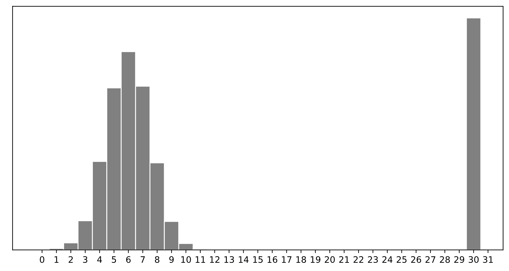
Consider a dataset of n integers, y_1, y_2, ..., y_n, whose histogram is given below:
Which of the following is closest to the constant prediction h^* that minimizes:
\displaystyle \frac{1}{n} \sum_{i = 1}^n \begin{cases} 0 & y_i = h \\ 1 & y_i \neq h \end{cases}
1
5
6
7
11
15
30
30.
The minimizer of empirical risk for the constant model when using zero-one loss is the mode.
Which of the following is closest to the constant prediction h^* that minimizes: \displaystyle \frac{1}{n} \sum_{i = 1}^n |y_i - h|
1
5
6
7
11
15
30
7.
The minimizer of empirical risk for the constant model when using absolute loss is the median. If the bar at 30 wasn’t there, the median would be 6, but the existence of that bar drags the “halfway” point up slightly, to 7.
Which of the following is closest to the constant prediction h^* that minimizes: \displaystyle \frac{1}{n} \sum_{i = 1}^n (y_i - h)^2
1
5
6
7
11
15
30
11.
The minimizer of empirical risk for the constant model when using squared loss is the mean. The mean is heavily influenced by the presence of outliers, of which there are many at 30, dragging the mean up to 11. While you can’t calculate the mean here, given the large right tail, this question can be answered by understanding that the mean must be larger than the median, which is 7, and 11 is the next biggest option.
Which of the following is closest to the constant prediction h^* that minimizes: \displaystyle \lim_{p \rightarrow \infty} \frac{1}{n} \sum_{i = 1}^n |y_i - h|^p
1
5
6
7
11
15
30
15.
The minimizer of empirical risk for the constant model when using infinity loss is the midrange, i.e. halfway between the min and max.
Source: Spring 2024 Final, Problem 2
Consider a dataset of 3 values, y_1 < y_2 < y_3, with a mean of 2. Let Y_\text{abs}(h) = \frac{1}{3} \sum_{i = 1}^3 |y_i - h| represent the mean absolute error of a constant prediction h on this dataset of 3 values.
Similarly, consider another dataset of 5 values, z_1 < z_2 < z_3 < z_4 < z_5, with a mean of 12. Let Z_\text{abs}(h) = \frac{1}{5} \sum_{i = 1}^5 |z_i - h| represent the mean absolute error of a constant prediction h on this dataset of 5 values.
Suppose that y_3 < z_1, and that T_\text{abs}(h) represents the mean absolute error of a constant prediction h on the combined dataset of 8 values, y_1, ..., y_3, z_1, ..., z_5.
Fill in the blanks:
“{ i } minimizes Y_\text{abs}(h), { ii } minimizes Z_\text{abs}(h), and { iii } minimizes T_\text{abs}(h).”
y_1
any value between y_1 and y_2 (inclusive)
y_2
y_3
z_1
z_1
z_2
any value between z_2 and z_3 (inclusive)
any value between z_2 and z_4 (inclusive)
z_3
y_2
y_3
any value between y_3 and z_1 (inclusive)
any value between z_1 and z_2 (inclusive)
any value between z_2 and z_3 (inclusive)
The values of the three blanks are: y_2, z_3, and any value between z_1 and z_2 (inclusive).
For the first blank, we know the median of the y-dataset minimizes mean absolute error of a constant prediction on the y-dataset. Since y_1 < y_2 < y_3, y_2 is the unique minimizer.
For the second blank, we can also use the fact that the median of the z-dataset minimizes mean absolute error of a constant prediction on the z-dataset. Since z_1 < z_2 < z_3 < z_4 < z_5, z_3 is the unique minimizer.
For the third blank, we know that when there are an odd number of data points in a dataset, any values between the middle two (inclusive) minimize mean absolute error. Here, the middle two in the full dataset of 8 are z_1 and z_2.
For any h, it is true that:
T_\text{abs}(h) = \alpha Y_\text{abs}(h) + \beta Z_\text{abs}(h)
for some constants \alpha and \beta. What are the values of \alpha and \beta? Give your answers as integers or simplified fractions with no variables.
\alpha = \frac{3}{8}, \beta = \frac{5}{8}.
To find \alpha and \beta, we need to construct a similar-looking equation to the one above. We can start by looking at our equation for T_\text{abs}(h):
T_\text{abs}(h) = \frac{1}{8} \sum_{i = 1}^8 |t_i - h|
Now, we can split the sum on the right hand side into two sums, one for our y data points and one for our z data points:
T_\text{abs}(h) = \frac{1}{8} \left(\sum_{i = 1}^3 |y_i - h| + \sum_{i = 1}^5 |z_i - h|\right)
Each of these two mini sums can be represented in terms of Y_\text{abs}(h) and Z_\text{abs}(h):
T_\text{abs}(h) = \frac{1}{8} \left(3 \cdot Y_\text{abs}(h) + 5 \cdot Z_\text{abs}(h)\right) T_\text{abs}(h) = \frac38 \cdot Y_\text{abs}(h) + \frac58 \cdot Z_\text{abs}(h)
By looking at this final equation we’ve built, it is clear that \alpha = \frac{3}{8} and \beta = \frac{5}{8}.
Show that Y_\text{abs}(z_1) = z_1 - 2.
Hint: Use the fact that you know the mean of y_1, y_2, y_3.
We can start by plugging z_1 into Y_\text{abs}(h):
Y_\text{abs}(z_1) = \frac{1}{3} \left( | z - y_1 | + | z - y_2 | + |z - y_3| \right)
Since z_1 > y_3 > y_2 > y_1, all of the absolute values can be dropped and we can write:
Y_\text{abs}(z_1) = \frac{1}{3} \left( (z_1 - y_1) + (z_1 - y_2) + (z_3 - y_3) \right)
This can be simplified to:
Y_\text{abs}(h) = \frac{1}{3} \left( 3z_1 - (y_1 + y_2 + y_3) \right) = \frac{1}{3} \left( 3z_1 - 3 \cdot \bar{y}\right) = z_1 - \bar{y} = z_1 - 2.
Suppose the mean absolute deviation from the median in the full dataset of 8 values is 6. What is the value of z_1?
Hint: You’ll need to use the results from earlier parts of this question.
2
3
5
6
7
9
11
3.
We are given that T_\text{abs}(\text{median}) = 6. This means that any value (inclusive) between z_1 and z_2 minimize T_\text{abs}(h), with the output being always being 6. So, T_\text{abs}(z_1) = 6. Let’s see what happens when we plug this into T_\text{abs}(h) = \frac{3}{8} Y_\text{abs}(h) + \frac{5}{8} Z_\text{abs}(h) from earlier:
T_\text{abs}(z_1) = \frac{3}{8} Y_\text{abs}(z_1) + \frac{5}{8} Z_\text{abs}(z_1) (6) = \frac{3}{8} Y_\text{abs}(z_1) + \frac{5}{8} Z_\text{abs}(z_1)
If we could write Y_\text{abs}(z_1) and Z_\text{abs}(z_1) in terms of z_1, we could solve for z_1 and our work would be done, so let’s do that. Y_\text{abs}(z_1) = z_1 - 2 from earlier. Z_\text{abs}(z_1) simplifies as follows (knowing that \bar{z} = 12):
Z_\text{abs}(z_1) = \frac{1}{5} \sum_{i = 1}^5 |z_i - z_1| Z_\text{abs}(z_1) = \frac{1}{5} \left(|z_1 - z_1| + |z_2 - z_1| + |z_3 - z_1| + |z_4 - z_1| + |z_5 - z_1|\right) Z_\text{abs}(z_1) = \frac{1}{5} \left(0 + (z_2 + z_3 + z_4 + z_5) - 4z_1\right) Z_\text{abs}(z_1) = \frac{1}{5} \left((z_2 + z_3 + z_4 + z_5) - 4z_1 + (z_1 - z_1)\right) Z_\text{abs}(z_1) = \frac{1}{5} \left((z_1 + z_2 + z_3 + z_4 + z_5) - 5z_1\right) Z_\text{abs}(z_1) = \bar{z} - z_1 Z_\text{abs}(z_1) = (12) - z_1
Subbing back into our main equation:
(6) = \frac{3}{8} Y_\text{abs}(z_1) + \frac{5}{8} Z_\text{abs}(z_1) 6 = \frac{3}{8}(z_1 - 2) + \frac{5}{8}(12 - z_1) z_1 = 3
Source: Spring 2024 Final, Problem 3
Suppose we’re given a dataset of n points, (x_1, y_1), (x_2, y_2), ..., (x_n, y_n), where \bar{x} is the mean of x_1, x_2, ..., x_n and \bar{y} is the mean of y_1, y_2, ..., y_n.
Using this dataset, we create a transformed dataset of n points, (x_1', y_1'), (x_2', y_2'), ..., (x_n', y_n'), where:
x_i' = 4x_i - 3 \qquad y_i' = y_i + 24
That is, the transformed dataset is of the form (4x_1 - 3, y_1 + 24), ..., (4x_n - 3, y_n + 24).
We decide to fit a simple linear hypothesis function H(x') = w_0 + w_1x' on the transformed dataset using squared loss. We find that w_0^* = 7 and w_1^* = 2, so H^*(x') = 7 + 2x'.
Suppose we were to fit a simple linear hypothesis function through the original dataset, (x_1, y_1), (x_2, y_2), ..., (x_n, y_n), again using squared loss. What would the optimal slope be?
2
4
6
8
11
12
24
8.
Relative to the dataset with x', the dataset with x has an x-variable that’s “compressed” by a factor of 4, so the slope increases by a factor of 4 to 2 \cdot 4 = 8.
Concretely, this can be shown by looking at the formula 2 = r\frac{SD(y')}{SD(x')}, recognizing that SD(y') = SD(y) since the y values have the same spread in both datasets, and that SD(x') = 4 SD(x).
Recall, the hypothesis function H^* was fit on the transformed dataset,
(x_1', y_1'), (x_2', y_2'), ..., (x_n', y_n'). H^* happens to pass through the point (\bar{x}, \bar{y}). What is the value of \bar{x}? Give your answer as an integer with no variables.
5.
The key idea is that the regression line always passes through (\text{mean } x, \text{mean } y) in the dataset we used to fit it. So, we know that: 2 \bar{x'} + 7 = \bar{y'}. This first equation can be rewritten as: 2 \cdot (4\bar{x} - 3) + 7 = \bar{y} + 24.
We’re also told this line passes through (\bar{x}, \bar{y}), which means that it’s also true that: 2 \bar{x} + 7 = \bar{y}.
Now we have a system of two equations:
\begin{cases} 2 \cdot (4\bar{x} - 3) + 7 = \bar{y} + 24 \\ 2 \bar{x} + 7 = \bar{y} \end{cases}
\dots and solving our system of two equations gives: \bar{x} = 5.
Source: Spring 2024 Final, Problem 4
Consider the vectors \vec{u} and \vec{v}, defined below.
\vec{u} = \begin{bmatrix} 1 \\ 0 \\ 0 \end{bmatrix} \qquad \vec{v} = \begin{bmatrix} 0 \\ 1 \\ 1 \end{bmatrix}
We define X \in \mathbb{R}^{3 \times 2} to be the matrix whose first column is \vec u and whose second column is \vec v.
In this part only, let \vec{y} = \begin{bmatrix} -1 \\ k \\ 252 \end{bmatrix}.
Find a scalar k such that \vec{y} is in \text{span}(\vec u, \vec v). Give your answer as a constant with no variables.
252.
Vectors in \text{span}(\vec u, \vec v) must have an equal 2nd and 3rd component, and the third component is 252, so the second must be as well.
Show that: (X^TX)^{-1}X^T = \begin{bmatrix} 1 & 0 & 0 \\ 0 & \frac{1}{2} & \frac{1}{2} \end{bmatrix}
Hint: If A = \begin{bmatrix} a_1 & 0 \\ 0 & a_2 \end{bmatrix}, then A^{-1} = \begin{bmatrix} \frac{1}{a_1} & 0 \\ 0 & \frac{1}{a_2} \end{bmatrix}.
We can construct the following series of matrices to get (X^TX)^{-1}X^T.
In parts (c) and (d) only, let \vec{y} = \begin{bmatrix} 4 \\ 2 \\ 8 \end{bmatrix}.
Find scalars a and b such that a \vec u + b \vec v is the vector in \text{span}(\vec u, \vec v) that is as close to \vec{y} as possible. Give your answers as constants with no variables.
a = 4, b = 5.
The result from the part (b) implies that when using the normal equations to find coefficients for \vec u and \vec v – which we know from lecture produce an error vector whose length is minimized – the coefficient on \vec u must be y_1 and the coefficient on \vec v must be \frac{y_2 + y_3}{2}. This can be shown by taking the result from part (b), \begin{bmatrix} 1 & 0 & 0 \\ 0 & \frac{1}{2} & \frac{1}{2} \end{bmatrix}, and multiplying it by the vector \vec y = \begin{bmatrix} y_1 \\ y_2 \\ y_3 \end{bmatrix}.
Here, y_1 = 4, so a = 4. We also know y_2 = 2 and y_3 = 8, so b = \frac{2+8}{2} = 5.
Let \vec{e} = \vec{y} - (a \vec u + b \vec v), where a and b are the values you found in part (c).
What is \lVert \vec{e} \rVert?
0
3 \sqrt{2}
4 \sqrt{2}
6
6 \sqrt{2}
2\sqrt{21}
3 \sqrt{2}.
The correct value of a \vec u + b \vec v = \begin{bmatrix} 4 \\ 5 \\ 5\end{bmatrix}. Then, \vec{e} = \begin{bmatrix} 4 \\ 2 \\ 8 \end{bmatrix} - \begin{bmatrix} 4 \\ 5 \\ 5 \end{bmatrix} = \begin{bmatrix} 0 \\ -3 \\ 3 \end{bmatrix}, which has a length of \sqrt{0^2 + (-3)^2 + 3^2} = 3\sqrt{2}.
Is it true that, for any vector \vec{y} \in \mathbb{R}^3, we can find scalars c and d such that the sum of the entries in the vector \vec{y} - (c \vec u + d \vec v) is 0?
Yes, because \vec{u} and \vec{v} are linearly independent.
Yes, because \vec{u} and \vec{v} are orthogonal.
Yes, but for a reason that isn’t listed here.
No, because \vec{y} is not necessarily in
No, because neither \vec{u} nor \vec{v} is equal to the vector
No, but for a reason that isn’t listed here.
Yes, but for a reason that isn’t listed here.
Here’s the full reason: 1. We can use the normal equations to find c and d, no matter what \vec{y} is. 2. The error vector \vec e that results from using the normal equations is such that \vec e is orthogonal to the span of the columns of X. 3. The columns of X are just \vec u and \vec v. So, \vec e is orthogonal to any linear combination of \vec u and \vec v. 4. One of the many linear combinations of \vec u and \vec v is \begin{bmatrix} 1 \\ 0 \\ 0 \end{bmatrix} + \begin{bmatrix} 0 \\ 1 \\ 1 \end{bmatrix} = \begin{bmatrix} 1 \\ 1 \\ 1 \end{bmatrix}. 5. This means that the vector \vec e is orthogonal to \begin{bmatrix} 1 \\ 1 \\ 1 \end{bmatrix}, which means that \vec{1}^T \vec{e} = 0 \implies \sum_{i = 1}^3 e_i = 0.
Suppose that Q \in \mathbb{R}^{100 \times 12}, \vec{s} \in \mathbb{R}^{100}, and \vec{f} \in \mathbb{R}^{12}. What are the dimensions of the following product?
\vec{s}^T Q \vec{f}
scalar
12 \times 1 vector
100 \times 1 vector
100 \times 12 matrix
12 \times 12 matrix
12 \times 100 matrix
undefined
Correct: Scalar.
The inner dimensions of 100 and 12 cancel, and so \vec{s}^T Q \vec{f} is of shape 1 x 1.
Source: Spring 2024 Final, Problem 7
Delta has released a line of trading cards. Each trading card has a picture of a plane and a color. There are 12 plane types, and for each plane type there are three possible colors (gold, silver, and platinum), meaning there are 36 trading cards total.
After your next flight, a pilot hands you a set of 6 cards, drawn at random without replacement from the set of 36 possible cards. The order of cards in a set does not matter.
In this question, you may leave your answers unsimplified, in terms of fractions, exponents, the permutation formula P(n, k), and the binomial coefficient {n \choose k}.
How many sets of 6 cards are there in total?
{36 \choose 6} = \frac{36!}{6!30!} = \frac{36 \cdot 35 \cdot 34 \cdot 33 \cdot 32 \cdot 31}{6!} = \frac{P(36, 6)}{6!}. Any of these answers, or anything equivalent to them, are correct.
There are 36 cards, and we must choose of 6 of them at random without replacement such that order matters.
How many sets of 6 cards have exactly 6 unique plane types?
{12 \choose 6} \cdot 3^6. Anything equivalent to this answer is also correct.
Since we’re asking for the number of hands with unique types, we first pick 6 different types, which can be done {12 \choose 6} ways. Then, for each chosen type, there are {3 \choose 1} = 3 ways of selecting the color. So, the colors can be chosen in 3 \cdot 3 \cdot ... \cdot 3 = 3^6 ways.
How many sets of 6 cards have exactly 2 unique plane types?
{12 \choose 2} = 66. Anything equivalent to this answer is also correct.
Once we pick 2 unique plane types, we need to choose 3 different colors per type, out of a set of 3 possibilities. This can be done, for each type, in {3 \choose 3} = 1 way.
How many sets of 6 cards have exactly 3 unique plane types, such that each plane type appears twice?
{12 \choose 3} \cdot {3 \choose 2}^3 = {12 \choose 3} 3^3. Anything equivalent to this answer is also correct.
First, we choose 3 distinct types, which can be done in ${12 \choose 3} ways. Then, for each type, we choose 2 colors, which can be done in {3 \choose 2} ways per type.
How many sets of 6 cards have exactly 3 unique plane types?
Hint: You’ll need to consider multiple cases, one of which you addressed in part (d).
{12 \choose 3} \cdot {3 \choose 2}^3 + {12 \choose 1}{11 \choose 1}{3 \choose 2}{10 \choose 1}{3 \choose 1}. Anything equivalent to this answer is also correct.
If we select 6 cards and end up with 3 unique plane types, there are two possibilities: - We get 2 of each type (e.g. xx yy zz). This is the case in part (d), so the total number of sets of 6 cards that fall here are {12 \choose 3} \cdot {3 \choose 2}^3. - We get 3 of one type, 2 of another, and 1 of the last one (e.g. xxx yy z). - xxx: There are 12 options for the type that appears 3 times, so that can be selected in {12 \choose 1} ways. We must take all 3 of that types colors, which can be done in {3 \choose 3} = 1 way. - yy: There are now 11 options for the type that appears 2 times, and for that type, we must take 2 of its three colors, so there are {11 \choose 1}{3 \choose 2} options. - z: There are now 10 options for the type that appears once, and for that type, we must take 1 of its three colors, so there are {10 \choose 1}{3 \choose 1} options. - So, the total number of options for this case is {12 \choose 1}{11 \choose 1}{3 \choose 2}{10 \choose 1}{3 \choose 1} = P(12, 3) 3^2 = {12 \choose 3} 3^3 \cdot 2.
So, the total number of options is {12 \choose 3} \cdot {3 \choose 2}^3 + {12 \choose 1}{11 \choose 1}{3 \choose 2}{10 \choose 1}{3 \choose 1}, which can be simplified in various ways, including to {12 \choose 3}3^4. Any of these ways received full credit, as long as they showed all work and logic.
Source: Fall 2021 Midterm, Problem 1
King Triton just made an Instagram account and has been keeping track of the number of likes his posts have received so far.
His first 7 posts have received a mean of 16 likes; the specific like counts in sorted order are
8, 12, 12, 15, 18, 20, 27
King Triton wants to predict the number of likes his next post will receive, using a constant prediction rule h. For each loss function L(h, y), determine the constant prediction h^* that minimizes empirical risk. If you believe there are multiple minimizers, specify them all. If you believe you need more information to answer the question or that there is no minimizer, state that clearly. Give a brief justification for each answer.
L(h, y) = |y - h|
This is absolute loss, and hence we’re looking for the minimizer of mean absolute error, which is the median, 15.
L(h, y) = (y - h)^2
This is squared loss, and hence we’re looking for the minimizer of mean squared error, which is the mean, 16.
L(h, y) = 4(y - h)^2
This is squared loss, multiplied by a constant. Note that when we go to minimize empirical risk for this loss function, we will take the derivative of empirical risk and set it equal to 0; at that point the constant factor of 4 can be divided from both sides, so this problem boils down to minimizing ordinary mean squared error. The only difference is that the graph of mean squared error will be stretched vertically by a factor of 4; the minimizing value will be in the same place.
For more justification, here we consider any general re-scaling \alpha (y-h)^2:
\begin{aligned} R_{sq}(h) &= \frac{1}{n} \sum_{i = 1}^n \alpha (y_i - h)^2 \\ &= \alpha \cdot \frac{1}{n} \sum_{i = 1}^n (y_i - h)^2 \\ \frac{d}{dh} R_{sq}(h) &= \alpha \cdot \frac{1}{n} \sum_{i = 1}^n 2(y_i - h)(-1) = 0\\ &\implies -\frac{2\alpha}{n}\sum_{i = 1}^n (y_i - h) = 0 \\ &\implies \sum_{i = 1}^n (y_i - h) = 0 \\ &\implies h^* = \frac{1}{n} \sum_{i = 1}^n y_i \end{aligned}
L(h, y) = \begin{cases} 0 & h = y \\ 100 & h \neq y \end{cases}
This is a scaled version of 0-1 loss. We know that empirical risk for 0-1 loss is minimized at the mode, so that also applies here. The mode, i.e. the most common value, is 12.
L(h, y) = (3y - 4h)^2
Note that we can write (3y - 4h)^2 as \left( 3 \left( y - \frac{4}{3}h \right) \right)^2 = 9 \left( y - \frac{4}{3}h \right)^2. As we’ve seen, the constant factor out front has no impact on the minimizing value. Using the same principle as in the last part, we can say that \frac{4}{3} h^* = \bar{x} \implies h^* = \frac{3}{4} \bar{x} = \frac{3}{4} \cdot 16 = 12
L(h, y) = (y - h)^3
Hint: Do not spend too long on this subpart.
No minimizer.
Note that unlike |y - h|, (y - h)^2, and all of the other loss functions we’ve seen, (y - h)^3 tends towards -\infty, rather than having a minimum output of 0. This means that there is no h that minimizes \frac{1}{n} \sum_{i = 1}^n (y_i - h)^3; the larger we make h, the more negative (and hence “smaller") this empirical risk becomes.
Source: Fall 2021 Midterm, Problem 2
Consider a set of 23 data points y_1, y_2, y_3, ..., y_{23} such that y_1 < y_2 < ... < y_{23}. Let’s call this Dataset A.
We create a new dataset, Dataset B, by repeating each point in Dataset A once. That is, Dataset B is the set of 46 points y_1, y_1, y_2, y_2, ..., y_{23}, y_{23}.
Answer the following questions regarding the relationship between Dataset A and Dataset B. Justify your answers.
Suppose the minimizer of mean absolute error R_{abs}(h) for Dataset A is 5. What is the minimizer of mean absolute error for Dataset B? If you believe there are multiple minimizers, specify them all. If you believe you need more information to answer the question, state that clearly.
The minimizer of MAE for Dataset B is still 5.
Note that when we repeat each data point, we go from having an odd number of data points (23) to an even number (46). This means the minimizer is the set of all values between the middle two values. But the middle two values will now both be y_{12}, and so there are no numbers “in between" them – only y_{12} minimizes MAE.
Suppose the mean absolute deviation from the median for Dataset A is 17. What is the mean absolute deviation from the median for Dataset B? If you believe you need more information to answer the question, state that clearly.
The mean absolute deviation from the median for Dataset B is still 17.
As we saw in previous part, the median itself does not change. When adding together the deviations from the median, each point is repeated twice, so the sum of all deviations from the median is doubled. However, there are twice as many data points in Dataset B than there are in Dataset A, so we divide by 2n (46) instead of n (23) in our average.
In short, for Dataset B both the numerator and denominator in the calculation of mean absolute deviation from the median \frac{\sum_{i = 1}^n |y_i - \text{Median}(y)|}{n} are double what they were for Dataset A, so the end result is the same as for Dataset A.
Suppose the function R_A(h) represents mean absolute error for Dataset A and R_B(h) represents mean absolute error for Dataset B.
Is it true that R_A(h) = R_B(h) for any real number h? (In other words, are the graphs of R_A(h) and R_B(h) identical?) Explain your reasoning.
Yes, R_{A}(h) = R_{B}(h).
Recall that the definition of R_{abs}(h) is:
R_{abs}(h) = \frac{1}{n} \sum_{i = 1}^n |y_i - h|
For the first dataset, we have:
R_{A}(h) = \frac{1}{23} \sum_{i = 1}^{23} |y_i - h|
and for the second dataset, we have:
\begin{aligned} R_{B}(h) &= \frac{1}{46} \sum_{i = 1}^{46} \left( |y_1 - h| + |y_1 - h| + |y_2 - h| + |y_2 - h| + ... + |y_{23} - h| + |y_{23} - h| \right) \\ &= \frac{1}{46} \left( 2 \sum_{i = 1}^{23} |y_i - h| \right) \\ &= \frac{1}{23} \sum_{i = 1}^{23} |y_i - h| \\ &= R_{A}(h) \end{aligned}
Source: Fall 2021 Final Exam, Problem 1
The mean of 12 non-negative numbers is 45. Suppose we remove 2 of these numbers. What is the largest possible value of the mean of the remaining 10 numbers? Show your work.
54.
To maximize the mean of the remaining 10 numbers, we want to minimize the numbers that are removed. The smallest possible non-negative number is 0, so to maximize the mean of the remaining 10, we should remove two 0s from the set of numbers. Recall that the sum of the 12 number set is 12 \cdot 45; then, the maximum possible mean of the remaining 10 is
\frac{12 \cdot 45 - 2 \cdot 0}{10} = \frac{6}{5} \cdot 45 = 54
Source: Fall 2021 Final Exam, Problem 2
Consider a set of 8 data points, y_1, y_2, ..., y_8 that are in sorted order, i.e. y_1 < y_2 < ... < y_8. Suppose that y_4 = 10, y_5 = 14, and y_6 = 22. Recall that mean absolute error, R_{abs}(h), is defined as R_{abs}(h) = \frac{1}{n} \sum_{i = 1}^n |y_i - h|. Suppose that R_{abs}(11) = 9.
What is R_{abs}(22)? Show your work.
Hint: Use the formula for the slope of R at h.
R_{abs}(22) = 11
We can write the points given to us as:
y_1, y_2, y_3, 10, 14, 22, y_7, y_8
Since there are an even number of data points, all values of h between the middle two points minimize R_{abs}(h). In this case, all values of h in the interval [10, 14] minimize R_{abs}(h) and, as a result, have the same value of R_{abs}(h). Thus, R_{abs}(14) = R_{abs}(11) = 9.
From lecture, we know that:
\text{slope of $R$ at $h$} = \frac{1}{n} \left( \left(\text{\# points } < h\right) - \left(\text{\# points } > h\right)\right)
We can use this formula to determine what to add to R_{abs}(14) to get R_{abs}(22). For any h in the interval (14, 22), the slope of R at h (given by plugging any h \in (14, 22) into the slope equation)is \frac{1}{8} (5 - 3) = \frac{1}{4}. This means that for every 1 unit we move to the right from h = 14 until we get to h = 22, R_{abs}(h) increases by \frac{1}{4}. So,
R_{abs}(22) = R_{abs}(14) + (22 - 14) \cdot \frac{1}{4} = 9 + 2 = 11
You can visualize the solution to this problem with this interactive graph.
Source: Fall 2021 Final Exam, Problem 4
You may find the following properties of logarithms helpful in this question. Assume that all logarithms in this question are natural logarithms, i.e. of base e.
Billy, the avocado-farmer-turned-waiter-turned-Instagram-influencer that you’re all-too-familiar with, is trying his hand at coming up with loss functions. He comes up with the Billy loss, L_B(h, y), defined as follows:
L_B(h, y) = \left[ \log \left( \frac{y}{h} \right) \right]^2
Throughout this problem, assume that all ys are positive.
Show that: \frac{d}{dh} L_B(h, y) = - \frac{2}{h} \log \left( \frac{y}{h} \right)
\begin{align*} \frac{d}{dh} L_B(h, y) &= \frac{d}{dh} \left[ \log \left( \frac{y}{h} \right) \right]^2 \\ &= 2 \cdot \log \left( \frac{y}{h} \right) \cdot \frac{d}{dh} \log \left( \frac{y}{h} \right) \\ &= 2 \cdot \log \left( \frac{y}{h} \right) \cdot \frac{d}{dh} \left( \log(y) - \log(h) \right) \\ &= 2 \cdot \log \left( \frac{y}{h} \right) \cdot \left( - \frac{1}{h} \right) \\ &= -\frac{2}{h} \log \left( \frac{y}{h} \right) \end{align*}
Show that the constant prediction h^* that minimizes for Billy loss is:
h^* = \left(y_1 \cdot y_2 \cdot ... \cdot y_n \right)^{\frac{1}{n}}
You do not need to perform a second derivative test, but otherwise you must show your work.
Hint: To confirm that you’re interpreting the result correctly, h^* for the dataset 3, 5, 16 is (3 \cdot 5 \cdot 16)^{\frac{1}{3}} = 240^{\frac{1}{3}} \approx 6.214.
\begin{align*} R_B(h) &= \frac{1}{n} \sum_{i = 1}^n \left[ \log \left( \frac{y_i}{h} \right) \right]^2 \\ \frac{d}{dh} R_B(h) &= \frac{1}{n} \sum_{i = 1}^n \frac{d}{dh} \left[ \log \left( \frac{y_i}{h} \right) \right]^2 \\ &= \frac{1}{n} \sum_{i = 1}^n -\frac{2}{h} \log \left( \frac{y_i}{h} \right) \\ &= -\frac{2}{nh} \sum_{i = 1}^n \log \left( \frac{y_i}{h} \right) = 0 \\ 0 &= \sum_{i = 1}^n \log \left( \frac{y_i}{h} \right) = \sum_{i = 1}^n \left( \log(y_i) - \log(h)\right) \\ 0 &= \sum_{i = 1}^n \log(y_i) - \log(h) \sum_{i = 1}^n 1 \\ 0 &= \left( \log(y_1) + \log(y_2) + ... + \log(y_n) \right) - n \log(h) \\ \log(h^n) &= \log(y_1 \cdot y_2 \cdot ... \cdot y_n) \\ h^n &= y_1 \cdot y_2 \cdot ... \cdot y_n \\ h^* &= (y_1 \cdot y_2 \cdot ... \cdot y_n)^{\frac{1}{n}} \end{align*}
Source: Fall 2022 Midterm, Problem 3
Mahdi runs a local pastry shop near UCSD and sells traditional desert called Baklava. He bakes Baklavas every morning to keep his promise of providing fresh Baklavas to his customers daily. Here is the amount of Baklava he sold each day during last week in pounds(lb): y_1=100, y_2=110, y_3=75, y_4=90, y_5=105, y_6=90, y_7=25
Mahdi needs your help as a data scientist to suggest the best constant prediction (h^*) of daily sales that minimizes the empirical risk using L(h,y) as the loss function. Answer the following questions and give a brief justification for each part. This problem has many parts, if you get stuck, move on and come back later!
Let L(h,y)=|y-h|. What is h^*? (We’ll later refer to this prediction as h_1^*).
As we have seen in lectures, the median minimizes the absolute loss risk function. h^*_1=\text{Median}(y_1, \cdots, y_7).
Let L(h,y)=(y-h)^2. What is h^*? (We’ll later refer to this prediction as h_2^*).
As we have seen in lectures, the mean minimizes the square loss risk function. h^*_2=\text{Mean}(y_1, \cdots, y_7).
True or False: Removing y_1 and y_3 from the dataset does not change h_2^*.
True
False
False. It changes the mean from 85 to 84. (However, the median is not changed.)
Mahdi thinks that y_7 is an outlier. Hence, he asks you to remove y_7 and update your predictions in parts (a) and (b) accordingly. Without calculating the new predictions, can you justify which prediction changes more? h^*_1 or h_2^*?
Removing y_7 affects h_2^* more than h_1^*. This is because the mean squared loss is more sensitive to outliers than absolute loss, and removing data changes the mean more.
True or False: Let L(y,h)=|y-h|^3. You can use the Gradient descent algorithm to find h^*.
True
False
False. The function |y-h|^3 is not differentiable everywhere so we can not use the gradient descent to find the minimum.
True or False: Let L(y,h)=\sin(y-h). The Gradient descent
algorithm is guaranteed to converge, provided that a proper learning
rate is given.
True
False
False. The function is not convex, so the gradient descent algorithm is not guaranteed to converge.
Mahdi has noticed that Baklava daily sale is associated with weather temperature. So he asks you to incorporate this feature to get a better prediction. Suppose the last week’s daily temperatures are x_1, x_2, \cdots, x_7 in Fahrenheit (F). We know that \bar x=65, \sigma_x=8.5 and the best linear prediction that minimizes the mean squared error is H^*(x)=-3x+w_0^*.
What is the correlation coefficient (r) between x and y? What does that mean?
r=-0.95. This means the weather temperature inversely affects Baklava sales, i.e., they are highly negatively correlated.
We know w_1^* = \frac{\sigma_y}{\sigma_x}r. We know that \sigma_x=8.5 and w_1^*=-3. We can find \sigma_y as follows:
\begin{aligned} \sigma_y^2 =& \frac{1}{n} \sum_{i = 1}^n (y_i - \bar{y})^2\\ =& \frac{1}{7}[(100-85)^2+(110-85)^2+(75-85)^2+(90-85)^2+(105-85)^2+(90-85)^2+(25-85)^2]\\ =&\frac{1}{7}[15^2+25^2+10^2+5^2+20^2+5^2+60^2]=714.28 \end{aligned}
Then, \sigma_y=26.7 which results in r=-0.95.
True or False: The unit of r is \frac{lb}{F} (Pound per Fahrenheit).
True
False
False. The correlation coefficient has no unit. (It is always a unitless number in [-1,1] range.)
Find w^*_0. (Hint: You’ll need to find \bar y for the given dataset)
w_0^*=280
Note that H(\bar x)=\bar y. Therefore, \begin{aligned} H(65)=-3\cdot 65 +w_0^*=85 \xrightarrow[]{}w_0^*=280. \end{aligned}
What would the best linear prediction H^*(x) be if we multiply all x_i’s by 2?
H^*(x) = -1.5x + 280
The standard deviation scales by a factor of 2, i.e., \sigma_x'=2\cdot \sigma_x.
The same
is true for the mean, i.e., \bar{x}'=2
\cdot \bar{x}.
The correlation r, standard deviation of the y-values \sigma_y, and the mean of the y-values \bar y do not change.
(You can verify
these claims by plugging 2x in for
x in their respective formulas and
seeing what happens, but it’s faster to visually reason why
this happens.)
Therefore, w_1'^*=\frac{\sigma_y'}{\sigma_x'}r' = \frac{(\sigma_y)}{(2\cdot\sigma_x)}(r) = \frac{w_1^*}{2} = -1.5.
We can find w_0'^* as follows:
\begin{align*} \bar{y}'&=H(\bar{x}')\\&=\frac{w_1^*}{2}(2\bar{x})+w_0'^*\\&=w_1^*\bar{x}+w_0'^* \\ &\downarrow \\ (85) &= -3(65) + w_0'^* \\ w_0'^*&=280 \end{align*}
So, H^*(x) would be -1.5x + 280.
What would the best linear prediction H^*(x) be if we add 20 to all x_i’s?
H^*(x) = -3x + 340
All parameters remain unchanged except \bar{x}'=\bar{x}+20. Since r, \sigma_x and \sigma_y are not changed, w_1^* does not change. Then, one can find w_0^* as follows:
\begin{align*} \bar{y}'&=H(\bar{x}') \\ &\downarrow \\ (85) &=-3(65+20)+w_0^* \\ w_0^*&=340 \end{align*}
So, H^*(x) would be -3x + 340.
Source: Fall 2022 Midterm, Problem 4
Consider a dataset that consists of y_1, \cdots, y_n. In class, we used calculus to minimize mean squared error, R_{sq}(h) = \frac{1}{n} \sum_{i = 1}^n (h - y_i)^2. In this problem, we want you to apply the same approach to a slightly different loss function defined below: L_{\text{midterm}}(y,h)=(\alpha y - h)^2+\lambda h
Write down the empiricial risk R_{\text{midterm}}(h) by using the above loss function.
R_{\text{midterm}}(h)=\frac{1}{n}\sum_{i=1}^{n}[(\alpha y_i - h)^2+\lambda h]=[\frac{1}{n}\sum_{i=1}^{n}(\alpha y_i - h)^2] +\lambda h
The mean of dataset is \bar{y}, i.e. \bar{y} = \frac{1}{n} \sum_{i = 1}^n y_i. Find h^* that minimizes R_{\text{midterm}}(h) using calculus. Your result should be in terms of \bar{y}, \alpha and \lambda.
h^*=\alpha \bar{y} - \frac{\lambda}{2}
\begin{align*} \frac{d}{dh}R_{\text{midterm}}(h)&= [\frac{2}{n}\sum_{i=1}^{n}(h- \alpha y_i )] +\lambda \\ &=2 h-2\alpha \bar{y} + \lambda. \end{align*}
By setting \frac{d}{dh}R_{\text{midterm}}(h)=0 we get 2 h^*-2\alpha \bar{y} + \lambda=0 \Rightarrow h^*=\alpha \bar{y} - \frac{\lambda}{2}.
Source: Spring 2023 Midterm 1, Problem 1
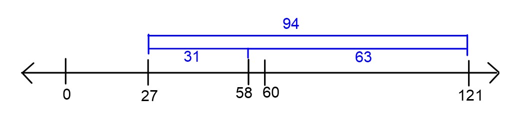
Consider a dataset such that 60 \leq y_1 \leq y_2 \leq \dots \leq y_n. Let R_{abs}(h) represent the mean absolute error of a constant prediction h on this dataset. Suppose we know that R_{abs}(27) = 94.
Find \bar y, or the mean of \{y_1, y_2, \dots, y_n\}.
\bar{y} = 121
There are several ways to complete this problem. One way is to interpret mean absolute error of a constant prediction h as the average distance of each data point to h. So we are told that the average distance of each data point to 27 is 94. That is, the data points are 94 units away from 27 on average. Since all the data is at least 60, they must be 94 units more than 27, or 121, on average.

You can also arrive at the same answer algebraically using the definition of R_{abs}(h). We have \begin{aligned} R_{abs}(h) &= \frac1n \sum_{i=1}^{n}|y_i - h| \\ R_{abs}(27) &= \frac1n \sum_{i=1}^{n}|y_i - 27| \\ &= \frac1n \sum_{i=1}^{n}(y_i - 27) \qquad \text{because each~} y_i\geq 60 \\ &= \frac1n\left( \sum_{i=1}^{n}y_i - \sum_{i=1}^{n}27\right) \\ &= \frac1n\left( n\cdot\bar y - n\cdot27\right) \\ &= \bar y - 27 \end{aligned}
Since we are told that R(27) = 94, we can set \bar y - 27 = 94, to find that \bar y = 121.
Find R_{abs}(58).
R_{abs}(58) = 63
Again, we can complete this problem in multiple ways. Interpreting R_{abs}(h) as the average distance of each data point to h, we can see that since 58 is 31 units closer to each data point than 27, R_{abs}(58) = R_{abs}(27) - 31 = 94 - 31 = 63.
Another way to do this problem uses the answer from part (a). Since the data points average to 121, their distance to 58 is 121-58 = 63, on average.
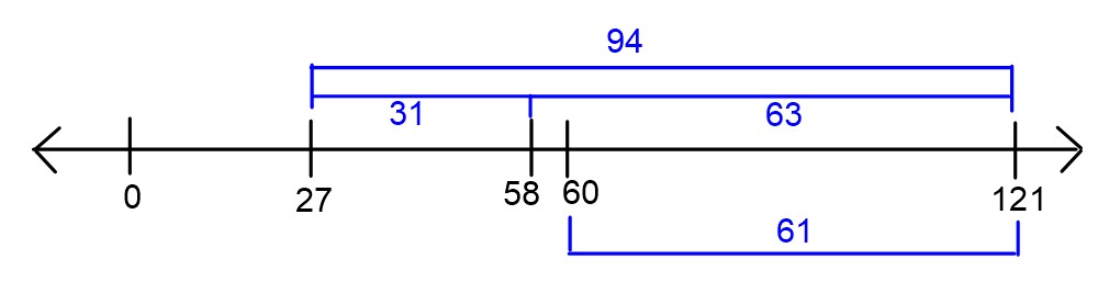
Which of the following could be the mean absolute deviation from the median for this dataset? There is only one correct answer.
18
62
94
102
Our answer is 18.
One easy way to do this problem is to recognize that none of these values are too low, but they may be too high. For example, the mean absolute deviation from the median can be as low as 0, when all the data points are the same. Since we are told there is only one correct answer and we know that no answer choice is too low, that means the correct answer must be the lowest option, 18.
We can also rule out all the other answer choices to show that they are too high. To do that, we’ll show that 62 is too high, and therefore, both 94 and 102 are too high as well. We are told that all data points are at least 60. By similar logic as we used in part (b), we can see that R_{abs}(60) = 61. Since the minimum value of R_{abs}(h) occurs at the median h^*\geq 60 and we already know R_{abs}(60) = 61, it must be the case that R(h^*) \leq 61.
Source: Spring 2023 Midterm 1, Problem 2
Let R_{sq}(h) represent the mean squared error of a constant prediction h for a given dataset. Find a dataset \{y_1, y_2\} such that the graph of R_{sq}(h) has its minimum at the point (7,16).
The dataset is {3, 11}.
We’ve already learned that R_{sq}(h) is minimized at the mean of the data, and the minimum value of R_sq(h) is the variance of the data. So we need to provide a dataset of two points with a mean of 7 and a variance of 16. Recall that the variance is the average squared distance of each data point to the mean. Since we want a variance of 16, we can make each point 4 units away from the mean. Therefore, our data set can be y_1 = 3, y_2 = 11. In fact, this is the only solution.
A more calculative approach uses the formulas for mean and variance and solves a system of two equations:
\begin{aligned} \frac{y_1+y_2}{2} &= 7 \\ \frac12 \left((y_1 - 7)^2 + (y_2 - 7)^2 \right) &= 16 \end{aligned}
Source: Spring 2023 Final Part 1, Problem 1
For a given dataset \{y_1, y_2, \dots, y_n\}, let M_{abs}(h) represent the median absolute error of the constant prediction h on that dataset (as opposed to the mean absolute error R_{abs}(h)).
For the dataset \{4, 9, 10, 14, 15\}, what is M_{abs}(9)?
5
The first step is to calculate the absolute errors (|y_i - h|).
\begin{align*} \text{Absolute Errors} &= \{|4-9|, |9-9|, |10-9|, |14-9|, |15-9|\} \\ \text{Absolute Errors} &= \{|-5|, |0|, |1|, |5|, |6|\} \\ \text{Absolute Errors} &= \{5, 0, 1, 5, 6\} \end{align*}
Now we have to order the values inside of the absolute errors: \{0, 1, 5, 5, 6\}. We can see the median is 5, so M_{abs}(9) =5.
For the same dataset \{4, 9, 10, 14, 15\}, find another integer h such that M_{abs}(9) = M_{abs}(h).
5 or 15
Our goal is to find another number that will give us the same median of absolute errors as in part (a).
One way to do this is to plug in a number and guess. Another way requires noticing you can modify 10 (the middle element) to become 5 in either direction (negative or positive) because of the absolute value.
We can solve this equation to get |10-x| = 5 \rightarrow x = 15 \text{ and } x = 5.
We can then test this by following the same steps as we did in part (a).
For x = 15: \begin{align*} \text{Absolute Errors} &= \{|4-15|, |9-15|, |10-15|, |14-15|, |15-15|\} \\ \text{Absolute Errors} &= \{|-11|, |-6|, |-5|, |-1|, |0|\} \\ \text{Absolute Errors} &= \{11, 6, 5, 1, 0\} \end{align*}
Then we order the elements to get the absolute errors: \{0, 1, 5, 6, 11\}. We can see the median is 5, so M_{abs}(15) =5.
For x = 5: \begin{align*} \text{Absolute Errors} &= \{|4-5|, |9-5|, |10-5|, |14-5|, |15-5|\} \\ \text{Absolute Errors} &= \{|-1|, |4|, |5|, |9|, |10|\} \\ \text{Absolute Errors} &= \{1, 4, 5, 9, 10\} \end{align*}
We do not have to re-order the elements because they are in order already. We can see the median is 5, so M_{abs}(5) =5.
Based on your answers to parts (a) and (b), discuss in at most two sentences what is problematic about using the median absolute error to make predictions.
The numbers 5 and 15 are clearly bad predictions (close to the extreme values in the dataset), yet they are considered just as good a prediction by this metric as the number 9, which is roughly in the center of the dataset. Intuitively, 9 is a much better prediction, but this way of measuring the quality of a prediction does not recognize that.
Source: Spring 2023 Final Part 1, Problem 2
Match each dataset with the graph of its mean absolute error, R_{abs}(h).
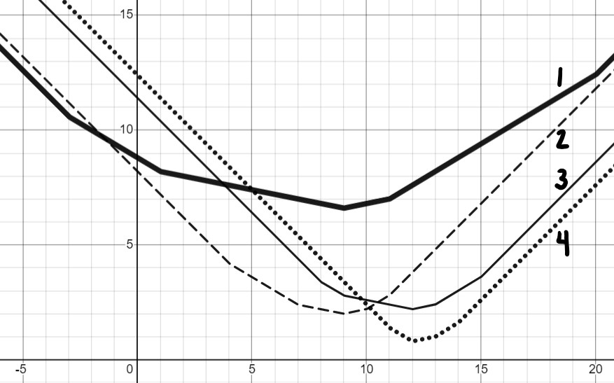
\{4, 7, 9, 10, 11\}
Graph 1
Graph 2
Graph 3
Graph 4
Graph 2
The important thing to note here is the y axis is equal to R_{abs}(h) and the x axis is equal to our h. The easiest way to figure out which graph belongs to which dataset is to choose some numbers for h and see if a line matches up with the chosen points.
| h^* | R_{abs}(h) |
|---|---|
| 0 | \frac{1}{5}\sum_{i = 1}^{5}|y_i-0| = \frac{1}{5} \cdot 41 \approx 8 |
| 8 | \frac{1}{5}\sum_{i = 1}^{5}|y_i-8| = \frac{1}{5} \cdot 11 = 2 |
| 18 | \frac{1}{5}\sum_{i = 1}^{5}|y_i-18| = \frac{1}{5} \cdot 49 \approx 10 |
When looking at these three places we can see that this dataset matches Graph 2.
\{-3, 1, 9, 11, 20\}
Graph 1
Graph 2
Graph 3
Graph 4
Graph 1
We will use the same approach we used in part (a).
| h^* | R_{abs}(h) |
|---|---|
| 0 | \frac{1}{5}\sum_{i = 1}^{5}|y_i-0| = \frac{1}{5} \cdot 44 \approx 9 |
| 8 | \frac{1}{5}\sum_{i = 1}^{5}|y_i-8| = \frac{1}{5} \cdot 34 \approx 7 |
| 18 | \frac{1}{5}\sum_{i = 1}^{5}|y_i-18| = \frac{1}{5} \cdot 56 \approx 11 |
When looking at these three places we can see that this dataset matches Graph 1.
\{8, 9, 12, 13, 15\}
Graph 1
Graph 2
Graph 3
Graph 4
Graph 3
We will use the same approach we used in the previous parts.
| h^* | R_{abs}(h) |
|---|---|
| 0 | \frac{1}{5}\sum_{i = 1}^{5}|y_i-0| = \frac{1}{5} \cdot 44 \approx 11 |
| 8 | \frac{1}{5}\sum_{i = 1}^{5}|y_i-8| = \frac{1}{5} \cdot 17 \approx 3 |
| 18 | \frac{1}{5}\sum_{i = 1}^{5}|y_i-18| = \frac{1}{5} \cdot 33 \approx 7 |
When looking at these three places we can see that this dataset matches Graph 3.
\{11, 12, 12, 13, 14\}
Graph 1
Graph 2
Graph 3
Graph 4
Graph 4
We will use the same approach we used in the previous parts.
| h^* | R_{abs}(h) |
|---|---|
| 0 | \frac{1}{5}\sum_{i = 1}^{5}|y_i-0| = \frac{1}{5} \cdot 62 \approx 12 |
| 8 | \frac{1}{5}\sum_{i = 1}^{5}|y_i-8| = \frac{1}{5} \cdot 22 \approx 4 |
| 18 | \frac{1}{5}\sum_{i = 1}^{5}|y_i-18| = \frac{1}{5} \cdot 28 \approx 6 |
When looking at these three places we can see that this dataset
matches Graph 4. Another way would be choosing the only option not
chosen in the other parts yet!
Source: Winter 2022 Midterm 1, Problem 1
Define the extreme mean (EM) of a dataset to be the average of its largest and smallest values. Let f(x)=-3x+4. Show that for any dataset x_1\leq x_2 \leq \dots \leq x_n, EM(f(x_1), f(x_2), \dots, f(x_n)) = f(EM(x_1, x_2, \dots, x_n)).
This linear transformation reverses the order of the data because if a<b, then -3a>-3b and so adding four to both sides gives f(a)>f(b). Since x_1\leq x_2 \leq \dots \leq x_n, this means that the smallest of f(x_1), f(x_2), \dots, f(x_n) is f(x_n) and the largest is f(x_1). Therefore,
\begin{aligned} EM(f(x_1), f(x_2), \dots, f(x_n)) &= \dfrac{f(x_n) + f(x_1)}{2} \\ &= \dfrac{-3x_n+4-3x_1+4}{2} \\ &= \dfrac{-3x_n-3x_1}{2} + 4\\ &= -3\left(\dfrac{x_1+x_n}{2}\right) + 4 \\ &= -3EM(x_1, x_2, \dots, x_n)+ 4\\ &= f(EM(x_1, x_2, \dots, x_n)). \end{aligned}
Source: Winter 2022 Midterm 1, Problem 2
Consider a new loss function, L(h, y) = e^{(h-y)^2}. Given a dataset y_1, y_2, \dots, y_n, let R(h) represent the empirical risk for the dataset using this loss function.
For the dataset \{1, 3, 4\}, calculate R(2). Simplify your answer as much as possible without a calculator.
R(2) = \frac13 (2e+e^4)
We need to calculate the loss for each data point then average the losses. That is, we need to calculate R(2) = \dfrac{1}{3} \sum_{i=1}^{3} e^{(2-y_i)^2}. The table below records the necessary information:
| y_i | 1 | 3 | 4 |
|---|---|---|---|
| 2-y_i | 1 | -1 | -2 |
| (2-y_i)^2 | 1 | 1 | 4 |
| e^{(2-y_i)^2} | e | e | e^4 |
This means: \begin{aligned} R(2) &= \dfrac{1}{3} \sum_{i=1}^{3} e^{(2-y_i)^2} \\ &= \frac13 (e+e+e^4) \\ &= \frac13 (2e+e^4) \end{aligned}
For the same dataset \{1, 3, 4\}, perform one iteration of gradient descent on R(h), starting at an initial prediction of h_0=2 with a step size of \alpha=\frac{1}{2}. Show your work and simplify your answer.
h_1 = 2 + \frac{2e^4}{3}
First, we calculate the derivative of R(h). Using the chain rule, we have \begin{align*} R(h) &= \dfrac1n \sum_{i=1}^n e^{(h-y_i)^2} \\ R'(h) &= \dfrac1n \sum_{i=1}^n e^{(h-y_i)^2}\cdot 2(h-y_i) \\ \end{align*} To apply the gradient descent update rule, we next have to calculate R'(h_0) or R'(2). Plugging in h=2 to the derivative we calculated above gives: \begin{align*} R'(2) &= \dfrac1n \sum_{i=1}^n e^{(2-y_i)^2}\cdot 2(2-y_i) \end{align*}
The table below records the necessary information (note that we’ve done most of the work already).
| y_i | 1 | 3 | 4 |
|---|---|---|---|
| 2-y_i | 1 | -1 | -2 |
| (2-y_i)^2 | 1 | 1 | 4 |
| e^{(2-y_i)^2} | e | e | e^4 |
| e^{(2-y_i)^2}\cdot 2(2-y_i) | 2e | -2e | -4e^4 |
Therefore: \begin{aligned} R'(2) &= \dfrac{1}{3} \sum_{i=1}^{3} e^{(2-y_i)^2\cdot 2(2-y_i)} \\ &= \frac13 (2e - 2e -4e^4) \\ &= \frac{-4e^4}{3}. \end{aligned} Applying the gradient descent update rule gives: \begin{aligned} h_1 &= h_0 - \alpha\cdot R'(h_0) \\ &= 2 - \frac{1}{2}\cdot \frac{-4e^4}{3} \\ &= 2 + \frac{2e^4}{3} \end{aligned}
Source: Winter 2023 Final, Problem 1
For each of the loss functions below, find the constant prediction h^* which minimizes the corresponding empirical risk with respect to the data y_1 = -3, y_2 = 2, y_3 = 2, y_4 = -2, y_5 = -6 .
The \alpha-absolute loss is defined as follows: L_{\alpha-\text{abs} }(h, y) = |h - (y-\alpha) |.
Use \alpha=3.
h^*=-2-3=-5
This is equivalent to the absolute loss on the same dataset shifted by \alpha. Therefore the optimal solution that minimizes this loss is the median (-2) shifted by -\alpha (-3).
Use \beta=2. Hint: plot the empirical risk function for y\in[-6, 3].
h^*=2 \cdot 2=4.
This is equivalent to the absolute loss on the same dataset scaled by \beta. Therefore the optimal solution that minimizes this loss is the mode scaled by \beta.
Source: Winter 2024 Final Part 1, Problem 1
Suppose there is a dataset containing 10000 integers:
Calculate the median of this dataset.
6
We know there is an even number of integers in this dataset because 10000 \% 2 = 0. We can find the middle of the dataset as follows: \frac{10000}{2} = 5000. This means the element in the 5000th position and 5001st position can give us our median. The element at the 5000th position is a 5 because 2500 + 2500 = 5000. The element at the 5001st position is a 7 because the next number after 5 is 7. We can then plug 5 and 7 into the equation: \frac{x_{5000} + x_{5001}}{2} = \frac{5 + 7}{2} = 6
How does the mean of this dataset compared to its median?
The mean is larger than the median
The mean is smaller than the median
The mean and the median are equal
The mean is smaller than the median.
We can calculate the mean as follows: \frac{2500 \cdot 3 + 2500 \cdot 5 + 4500 \cdot 7 + 500 \cdot 9}{10000} = 5.6 Using part (a) we know that 5.6 < 6, which means the mean is smaller than the median.
Source: Winter 2024 Midterm 1, Problem 1
Consider a dataset D with 5 data points \{7,5,1,2,a\}, where a is a positive real number. Note that a is not necessarily an integer.
Express the mean of D as a function of a, simplify the expression as much as possible.
\text{Mean($D$)} = \frac{a}{5} + 3
Depending on the range of a, the median of D could assume one of three possible values. Write out all possible median of D along with the corresponding range of a for each case. Express the ranges using double inequalities, e.g., i.e. 3<a\leq8:
\begin{cases} \text{Median($D$)} = 2 & \text{if a is in the range of } 0<a\leq2 \\ \text{Median($D$)} = a & \text{if a is in the range of } 2<a\leq5 \\ \text{Median($D$)} = 5 & \text{if a is in the range of } 5<a\leq\infty \\ \end{cases}
Determine the range of a that satisfies: \text{Mean}(D) < \text{Median}(D) Make sure to show your work.
\dfrac{15}{4}<a<10
Since there are 3 possible median
values, we will have to discuss each situation separately.
In case 1, when 0<a\leq2, \text{Median}(D) = 2. So, we have:
\begin{align*} \text{Mean}(D) &< \text{Median}(D)\\ 3 + \frac{a}{5} &< 2\\ a&<-5 \end{align*}
But a<-5 is in conflict with the condition 0<a\leq2, therefore there is no solution in this situation, and Median(D) = 2 is impossible.
In case 2, when 2<a<5, \text{Median}(D) = a. So, we have:
\begin{align*} \text{Mean}(D) &< \text{Median}(D)\\ 3 + \frac{a}{5} &< a\\ 3 &< \frac{4}{5} a\\ a &> \frac{15}{4}\\ \end{align*}
So a has to be larger than \frac{15}{4}. But remember from the prerequisite condition that 2<a<5.
To satisfy both conditions, we must have \frac{15}{4}<a<5.
In case 3, when a\geq5, \text{Median}(D) = 5. So, we have: \begin{align*} \text{Mean}(D) &< \text{Median}(D)\\ 3 + \frac{a}{5} &< 5\\ a&<10 \end{align*}
combining with the prerequisite condition, we have 5\leq a<10
Combining the range of all three cases, we have \dfrac{15}{4}<a<10 as our final answer.
Source: Winter 2024 Midterm 1, Problem 2
Let R_{sq}(h) represent the mean squared error of a constant prediction h for a given dataset. For the dataset \{3, y_{1}\}, the graph of R_{sq}(h) has its minimum at the point (5,r_{1}). Find out the value of y_{1} and r_{1}
y_1 = 7, r_1 = 4
The mean squared error is written as: \begin{align*} R_{sq}(h) = \frac{1}{n}\sum_{i=0}^{n}(y_{i}-h)^2 \end{align*}
Since we only have two data points (n=2), the equation simplifies to:
\begin{align*} R_{sq}(h) = \frac{1}{2}((y_{0}-h)^2+ (y_{1}-h)^2) \end{align*}
Taking the derivative with respect to h, we have: \begin{align*} \frac{dR_{sq}(h)}{dh} = -(y_{0}-h)- (y_{1}-h) \end{align*}
We know that the derivative has to be 0 at the local minima, therefore at h=5, we have:
\begin{align*} \frac{dR_{sq}(h)}{dh} = -(3-5)- (y_{1}-5) &= 0\\ % -2+y_1-5 &=0\\ y_1 &= 7 \end{align*}
So we know that the dataset is \{3,7\}. Given all these information, we can calculate r_1 with:
\begin{align*} R_{sq}(5) &= \frac{1}{2}((y_{0}-5)^2+ (y_{1}-5)^2)\\ &=\frac{1}{2}((3-5)^2+ (7-5)^2)\\ &=\frac{1}{2}(4+4)=4 \end{align*}
Source: Spring 2024 Final, Problem 1
Consider a dataset of n integers, y_1, y_2, ..., y_n, whose histogram is given below:
Which of the following is closest to the constant prediction h^* that minimizes:
\displaystyle \frac{1}{n} \sum_{i = 1}^n \begin{cases} 0 & y_i = h \\ 1 & y_i \neq h \end{cases}
1
5
6
7
11
15
30
30.
The minimizer of empirical risk for the constant model when using zero-one loss is the mode.
Which of the following is closest to the constant prediction h^* that minimizes: \displaystyle \frac{1}{n} \sum_{i = 1}^n |y_i - h|
1
5
6
7
11
15
30
7.
The minimizer of empirical risk for the constant model when using absolute loss is the median. If the bar at 30 wasn’t there, the median would be 6, but the existence of that bar drags the “halfway” point up slightly, to 7.
Which of the following is closest to the constant prediction h^* that minimizes: \displaystyle \frac{1}{n} \sum_{i = 1}^n (y_i - h)^2
1
5
6
7
11
15
30
11.
The minimizer of empirical risk for the constant model when using squared loss is the mean. The mean is heavily influenced by the presence of outliers, of which there are many at 30, dragging the mean up to 11. While you can’t calculate the mean here, given the large right tail, this question can be answered by understanding that the mean must be larger than the median, which is 7, and 11 is the next biggest option.
Which of the following is closest to the constant prediction h^* that minimizes: \displaystyle \lim_{p \rightarrow \infty} \frac{1}{n} \sum_{i = 1}^n |y_i - h|^p
1
5
6
7
11
15
30
15.
The minimizer of empirical risk for the constant model when using infinity loss is the midrange, i.e. halfway between the min and max.
Source: Spring 2024 Final, Problem 2
Consider a dataset of 3 values, y_1 < y_2 < y_3, with a mean of 2. Let Y_\text{abs}(h) = \frac{1}{3} \sum_{i = 1}^3 |y_i - h| represent the mean absolute error of a constant prediction h on this dataset of 3 values.
Similarly, consider another dataset of 5 values, z_1 < z_2 < z_3 < z_4 < z_5, with a mean of 12. Let Z_\text{abs}(h) = \frac{1}{5} \sum_{i = 1}^5 |z_i - h| represent the mean absolute error of a constant prediction h on this dataset of 5 values.
Suppose that y_3 < z_1, and that T_\text{abs}(h) represents the mean absolute error of a constant prediction h on the combined dataset of 8 values, y_1, ..., y_3, z_1, ..., z_5.
Fill in the blanks:
“{ i } minimizes Y_\text{abs}(h), { ii } minimizes Z_\text{abs}(h), and { iii } minimizes T_\text{abs}(h).”
y_1
any value between y_1 and y_2 (inclusive)
y_2
y_3
z_1
z_1
z_2
any value between z_2 and z_3 (inclusive)
any value between z_2 and z_4 (inclusive)
z_3
y_2
y_3
any value between y_3 and z_1 (inclusive)
any value between z_1 and z_2 (inclusive)
any value between z_2 and z_3 (inclusive)
The values of the three blanks are: y_2, z_3, and any value between z_1 and z_2 (inclusive).
For the first blank, we know the median of the y-dataset minimizes mean absolute error of a constant prediction on the y-dataset. Since y_1 < y_2 < y_3, y_2 is the unique minimizer.
For the second blank, we can also use the fact that the median of the z-dataset minimizes mean absolute error of a constant prediction on the z-dataset. Since z_1 < z_2 < z_3 < z_4 < z_5, z_3 is the unique minimizer.
For the third blank, we know that when there are an odd number of data points in a dataset, any values between the middle two (inclusive) minimize mean absolute error. Here, the middle two in the full dataset of 8 are z_1 and z_2.
For any h, it is true that:
T_\text{abs}(h) = \alpha Y_\text{abs}(h) + \beta Z_\text{abs}(h)
for some constants \alpha and \beta. What are the values of \alpha and \beta? Give your answers as integers or simplified fractions with no variables.
\alpha = \frac{3}{8}, \beta = \frac{5}{8}.
To find \alpha and \beta, we need to construct a similar-looking equation to the one above. We can start by looking at our equation for T_\text{abs}(h):
T_\text{abs}(h) = \frac{1}{8} \sum_{i = 1}^8 |t_i - h|
Now, we can split the sum on the right hand side into two sums, one for our y data points and one for our z data points:
T_\text{abs}(h) = \frac{1}{8} \left(\sum_{i = 1}^3 |y_i - h| + \sum_{i = 1}^5 |z_i - h|\right)
Each of these two mini sums can be represented in terms of Y_\text{abs}(h) and Z_\text{abs}(h):
T_\text{abs}(h) = \frac{1}{8} \left(3 \cdot Y_\text{abs}(h) + 5 \cdot Z_\text{abs}(h)\right) T_\text{abs}(h) = \frac38 \cdot Y_\text{abs}(h) + \frac58 \cdot Z_\text{abs}(h)
By looking at this final equation we’ve built, it is clear that \alpha = \frac{3}{8} and \beta = \frac{5}{8}.
Show that Y_\text{abs}(z_1) = z_1 - 2.
Hint: Use the fact that you know the mean of y_1, y_2, y_3.
We can start by plugging z_1 into Y_\text{abs}(h):
Y_\text{abs}(z_1) = \frac{1}{3} \left( | z - y_1 | + | z - y_2 | + |z - y_3| \right)
Since z_1 > y_3 > y_2 > y_1, all of the absolute values can be dropped and we can write:
Y_\text{abs}(z_1) = \frac{1}{3} \left( (z_1 - y_1) + (z_1 - y_2) + (z_3 - y_3) \right)
This can be simplified to:
Y_\text{abs}(h) = \frac{1}{3} \left( 3z_1 - (y_1 + y_2 + y_3) \right) = \frac{1}{3} \left( 3z_1 - 3 \cdot \bar{y}\right) = z_1 - \bar{y} = z_1 - 2.
Suppose the mean absolute deviation from the median in the full dataset of 8 values is 6. What is the value of z_1?
Hint: You’ll need to use the results from earlier parts of this question.
2
3
5
6
7
9
11
3.
We are given that T_\text{abs}(\text{median}) = 6. This means that any value (inclusive) between z_1 and z_2 minimize T_\text{abs}(h), with the output being always being 6. So, T_\text{abs}(z_1) = 6. Let’s see what happens when we plug this into T_\text{abs}(h) = \frac{3}{8} Y_\text{abs}(h) + \frac{5}{8} Z_\text{abs}(h) from earlier:
T_\text{abs}(z_1) = \frac{3}{8} Y_\text{abs}(z_1) + \frac{5}{8} Z_\text{abs}(z_1) (6) = \frac{3}{8} Y_\text{abs}(z_1) + \frac{5}{8} Z_\text{abs}(z_1)
If we could write Y_\text{abs}(z_1) and Z_\text{abs}(z_1) in terms of z_1, we could solve for z_1 and our work would be done, so let’s do that. Y_\text{abs}(z_1) = z_1 - 2 from earlier. Z_\text{abs}(z_1) simplifies as follows (knowing that \bar{z} = 12):
Z_\text{abs}(z_1) = \frac{1}{5} \sum_{i = 1}^5 |z_i - z_1| Z_\text{abs}(z_1) = \frac{1}{5} \left(|z_1 - z_1| + |z_2 - z_1| + |z_3 - z_1| + |z_4 - z_1| + |z_5 - z_1|\right) Z_\text{abs}(z_1) = \frac{1}{5} \left(0 + (z_2 + z_3 + z_4 + z_5) - 4z_1\right) Z_\text{abs}(z_1) = \frac{1}{5} \left((z_2 + z_3 + z_4 + z_5) - 4z_1 + (z_1 - z_1)\right) Z_\text{abs}(z_1) = \frac{1}{5} \left((z_1 + z_2 + z_3 + z_4 + z_5) - 5z_1\right) Z_\text{abs}(z_1) = \bar{z} - z_1 Z_\text{abs}(z_1) = (12) - z_1
Subbing back into our main equation:
(6) = \frac{3}{8} Y_\text{abs}(z_1) + \frac{5}{8} Z_\text{abs}(z_1) 6 = \frac{3}{8}(z_1 - 2) + \frac{5}{8}(12 - z_1) z_1 = 3
Source: Summer Session 1 2025 Midterm, Problem 3a-c
Let \{x_i\}_{i=1}^n be a training dataset of scalar values, and suppose we wish to use the constant model
f(c;\, x) = c,\qquad c\in\mathbb{R}.
In various situations it can be useful to emphasize some training examples over others (e.g., due to data quality). For this purpose, suppose \alpha_1, \alpha_2, \dotsc, \alpha_n > 0 are fixed positive weights which are understood as separate from the training data and model parameters.
Find a formula for the minimizer c_1^\ast of the risk function
R_{1}(c) = \frac{1}{n} \sum_{i=1}^n \alpha_i(c - x_i)^2.
Find a formula for the minimizer c_2^\ast of the risk function
R_{2}(c) = \frac{1}{n} \sum_{i=1}^n \alpha_i |c - x_i|.
Which risk function is more sensitive to outliers?