The plot should have a y-intercept at (0,1) with slope of -1 until (1,0), where it plateaus to zero.
← return to practice.dsc40a.com
Instructor(s): Gal Mishne
This exam was administered in person. Students had 180 minutes to take this exam.
Source: Winter 2023 Final, Problem 1
For each of the loss functions below, find the constant prediction h^* which minimizes the corresponding empirical risk with respect to the data y_1 = -3, y_2 = 2, y_3 = 2, y_4 = -2, y_5 = -6 .
The \alpha-absolute loss is defined as follows: L_{\alpha-\text{abs} }(h, y) = |h - (y-\alpha) |.
Use \alpha=3.
h^*=-2-3=-5
This is equivalent to the absolute loss on the same dataset shifted by \alpha. Therefore the optimal solution that minimizes this loss is the median (-2) shifted by -\alpha (-3).
Use \beta=2. Hint: plot the empirical risk function for y\in[-6, 3].
h^*=2 \cdot 2=4.
This is equivalent to the absolute loss on the same dataset scaled by \beta. Therefore the optimal solution that minimizes this loss is the mode scaled by \beta.
Source: Winter 2023 Final, Problem 2
Let f(x):\mathbb{R}\to\mathbb{R} be a convex function. f(x) is not necessarily differentiable. Use the definition of convexity to prove the following: \begin{aligned} 2f(2) \leq f(1)+f(3) \end{aligned}Here is the definition of convexity:
f(tx_{1}+(1-t)x_{2})\leq tf(x_{1})+(1-t)f(x_{2})
Since f(x) is a convex function, we know that this inequality is satisfied for all choices of x_1 and x_2 on the real number line and all choices of t \in [0, 1]. This problem boils down to finding a choice of x_1, x_2, and t to morph the definition of convexity into our desired inequality.
One such successful combination is x_1=1, x_2=3, and t=0.5. This makes tx_{1}+(1-t)x_{2}=0.5\cdot 1 + (1 - 0.5)\cdot 3=2. Therefore: f(tx_{1}+(1-t)x_{2})=f(2) \leq 0.5f(x_{1})+f(x_{2})=0.5 (f(1)+f(3)) 2f(2) \leq f(1)+f(3).
The strategy for these variable choices boils down to trying to make the left side of the definition of convexity “look more” like the left side of our desired inequality, and trying to make the right side of the definition of convexity “look more” like the right side of our desired inequality.
Source: Winter 2023 Final, Problem 3
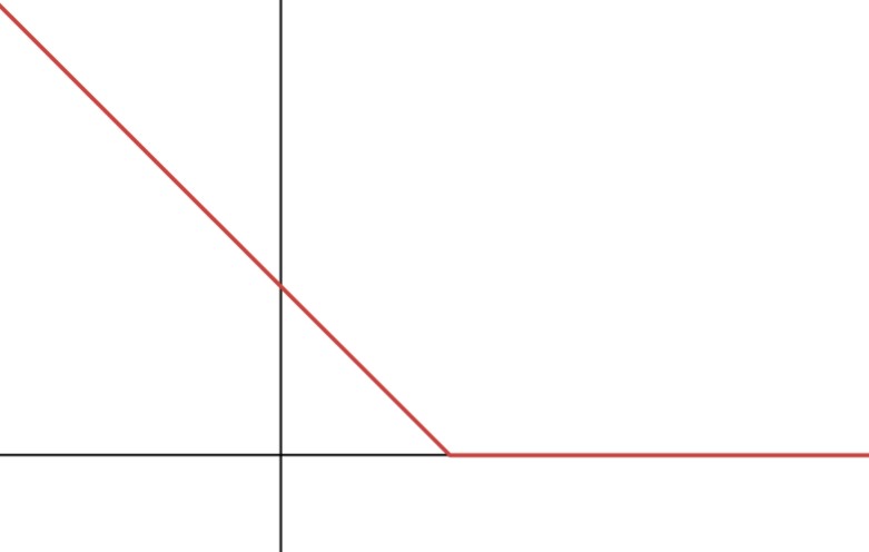
Let (x,y) be a sample where x is the feature and y denotes the class. Consider the following loss function, known as Hinge loss, for a predictor z of y: \begin{aligned} L(z)=\max(0,1-yz). \end{aligned}For all the following questions assume y=1.
Plot L(z).
The plot should have a y-intercept at (0,1) with slope of -1 until (1,0), where it plateaus to zero.
Is the global minima of L_s(z) unique?
The minima is not unique since the minimum value is 0 and any z\geq 1 achieves L(z)=0.
Perform two steps of gradient descent with step size \alpha=1 for L_s(z) starting from the point z_0=-0.5.
For z_0=-0.5, our point lies on the linear part of the function (L_s(z)=0.5-z), therefore {L'}_s(z)=-1. Our update is then: z_1=z_0 - \alpha {L'}_s(z_0)=-0.5+1=0.5
For z_1=0.5, our point lies on the quadratic part of the function (L_s(z)=0.5(1-z)^2), therefore {L'}_s(z)=-(1-z). The update is then z_2=z_1 - \alpha {L'}_s(z_1)=0.5+(1-0.5)=1
Source: Winter 2023 Final, Problem 4
Reggie and Essie are given a dataset of real features x_i \in \mathbb{R} and observations y_i. Essie proposes the following linear prediction rule: H_1(\alpha_0,\alpha_1) = \alpha_0 + \alpha_1 x_i. and Reggie proposes to use v_i=(x_i)^2 and the prediction rule H_2(\gamma_0,\gamma_1) = \gamma_0 + \gamma_1 v_i.
Give an example of a dataset \{(x_i,y_i)\}_{i=1}^n for which minimum MSE(H_2) < minimum MSE(H_1). Explain.
Example: If the datapoints follow a quadratic form y_i=x_i^2 for all i, then the H_2 prediction rule will achieve a zero error while H_1>0 since the data do not follow a linear form.
Give an example of a dataset \{(x_i,y_i)\}_{i=1}^n for which minimum MSE(H_2) = minimum MSE(H_1). Explain.
Example 1: If the response variables are constant y_i=c for all i, then for both prediciton rules by setting \alpha_0=\gamma_0=c and \alpha_1=\gamma_1=0, both predictors will achieve MSE=0.
Example 2: when every single value of the features x_i and x^2_ i coincide in the dataset (this occurs when x = 0 or x = 1), the parameters of both prediction rules will be the same, as will the MSE.
A new feature z has been added to the dataset.
Essie proposes a linear regression model using two predictor variables x,z as H_3(w_0,w_1,w_2) = w_0 + w_1 x_i +w_2 z_i.
Explain if the following statement is True or False (prove or provide counter-example).
Reggie claims that having more features will lead to a smaller error, therefore the following prediction rule will give a smaller MSE: H_4(\alpha_0,\alpha_1,\alpha_2,\alpha_3) = \alpha_0 + \alpha_1 x_i +\alpha_2 z_i + \alpha_3 (2x_i-z_i)
H_4 can be rewritten as H_4(\alpha_0,\alpha_1,\alpha_2,\alpha_3) = \alpha_0 + (\alpha_1+2\alpha_3) x_i +(\alpha_2 - \alpha_3)z_i By setting \tilde{\alpha}_1=\alpha_1+2\alpha_3 and \tilde{\alpha_2}= \alpha_2 - \alpha_3 then
H_4(\alpha_0,\alpha_1,\alpha_2,\alpha_3) = H_4(\alpha_0,\tilde{\alpha}_1,\tilde{\alpha}_2) = \alpha_0 + \tilde{\alpha_1} x_i +\tilde{\alpha}_2 z_i
Thus H_4 and H_3 have the same normal equations and therefore the same minimum MSE.
Source: Winter 2023 Final, Problem 5
Look at the following picture representing where the data are in a 2 dimensional space. We want to use k-means to cluster them into 3 groups. The cross shapes represent positions of the initial centroids (that are not data points).
Which of the following facts are true about the cluster assignment during the first iteration, as determined by these initial centroids (circle all answers that are correct)? All 35 circles are data points. All 3 plus-sign shapes are the initial centroids. Explain your selected answer(s).

Exactly one cluster contains 11 data points.
Exactly two clusters contain 11 data points.
Exactly one cluster contains at least 12 data points.
Exactly two clusters contain at least 12 data points.
None of the above.
Option 4 is correct.
The top cluster will contain 13 points. The left cluster will contain 10 points. The bottom right cluster will contain 12 points (including the outlier since it is closer to the bottom cross than to the left one). Therefore option 4 is correct.
The cross shapes represent positions of the initial centroids (that are not data points) before the first iteration. Now the algorithm is run for one iteration, where the centroids have been adjusted.
We are now starting the second iteration. Which of the following facts are true about the cluster assignment during the second iteration (circle all answers that are correct)? Explain your answer.
Exactly one cluster contains 11 data points.
Exactly two clusters contain 11 data points.
Exactly one cluster contains at least 12 data points.
Exactly two clusters contain at least 12 data points.
None of the above.
Options 2 and 3 are correct.
The top cluster will contain 13 points. The left cluster will contain 11 points (the outlier has now moved to this cluster since it will be closer to its centroid). The bottom right cluster will contain 11 points. Therefore options 2 and 3 are correct.
Compare the loss after the end of the second iteration to the loss at the end of the firs iteration. Which of the following facts are true (circle all answers that are correct)?
The loss at the end of the second iteration is lower.
The loss doesn’t decrease since there are actually 4 clusters in the data but we are using k-means with k=3.
The loss doesn’t decrease since there are actually 5 clusters in the data but we are using k-means with k=3.
The loss doesn’t decrease since there is an outlier that does not belong to any cluster.
The loss at the end of the second iteration is the same as at the end of the first iteration.
The loss at each iteration of k-means is non-increasing. Specifically, at the end of the second iteration the outlier having moved from the bottom right cluster to the left cluster will have decreased the loss.
Source: Winter 2023 Final, Problem 6
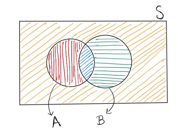
In the above figure, S is the sample space. Two events are denoted by two circles: A (Red + Blue) and B (Green + Blue). Which area denotes the event \bar{A}\cap\bar{B}?
Orange stripes
Red stripes
Green stripes
Blue stripes
Orange stripes.
\bar{A} is the area with green stripes and orange stripes. \bar{B} is the area with red stripes and orange stripes.
Therefore \bar{A}\cap\bar{B} is the area with orange stripes.
Use the law of total probability to prove De Morgan’s law: P(\bar{A}\cap\bar{B})=1-P(A\cup B). You may use the figure above to visualize the statement, but your proof must use the law of total probability.
We can write out the inclusion-exclusion principle. From there, we use the law of total probability to split up event B as the regions A\cap B and \bar{A}\cap B and continue from there:
\begin{align*} P(A\cup B)&=P({A}) + P({B}) - P(A\cap B)\\ &=P({A}) + \left[ P(A\cap B)+P(\bar{A}\cap B) \right]- P(A\cap B)\\ &=P({A}) + P(\bar{A}\cap B) \\ &=\left[ 1-P(\bar{A}) \right] + P(\bar{A}\cap B) \\ &=1- \left[P(\bar{A}\cap B) + P(\bar{A}\cap \bar{B}) \right] + P(\bar{A}\cap B)\\ &=1-P(\bar{A}\cap\bar{B}) \end{align*}
Therefore P(\bar{A}\cap\bar{B})=1-P(A\cup B).
Source: Winter 2023 Final, Problem 7
There is one box of bolts that contains some long and some short bolts. A manager is unable to open the box at present, so she asks her employees what is the composition of the box. One employee says that it contains 60 long bolts and 40 short bolts. Another says that it contains 10 long bolts and 20 short bolts. Unable to reconcile these opinions, the manager decides that each of the employees is correct with probability \frac{1}{2}. Let B_1 be the event that the box contains 60 long and 40 short bolts, and let B_2 be the event that the box contains 10 long and 20 short bolts. What is the probability that the first bolt selected is long?
P(\text{long}) = \frac{7}{15}
We are given that: P(B_1)=P(B_2)=\frac{1}{2} P(\text{long}|B_1) = \frac{60}{60 + 40} = \frac{3}{5} P(\text{long}|B_2) = \frac{10}{10 + 20} = \frac{1}{3}
Using the law of total probability:
P(\text{long})=P(\text{long}|B_1) \cdot P(B_1)+P(\text{long}|B_2) \cdot P(B_2) = \frac{3}{5} \cdot \frac{1}{2} + \frac{1}{3} \cdot \frac{1}{2} = \frac{7}{15}
How many ways can one arrange the letters A, B, C, D, E such that A, B, and C are all together (in any order)?
There are 3! \cdot 3! permutations.
We can treat the group of A, B, and C (in any order) as a single block of letters which we can call X. This will gurantee that any permutation we find will satisfy our condition of having A, B, and C being all together.
Our problem now has 3! = 6 permutations of our new letter bank: X, D, and E.
XDE XED DXE EXD DEX EDX
Let’s call these 6 permutations “structures”. For each of these structures, there are 3! = 6 rearrangements of the letters A, B, and C inside of X.
So, with 3! different arrangements of D, E and our block of letters (X), and with each of those arrangements individually having 3! ways to re-order the group of ABC, the overall number of permutations of ABCDE where ABC are all together, in any order, is 3! \cdot 3!.
Two chess players A and B play a series of chess matches against each other until one of them wins 3 matches. Every match ends when one of the players wins against the other, that is, the game does not ever end in draw/tie. For example, one series of matches ends when the outcomes of the first four games are: A wins, A wins, B wins, A wins. In how many different ways can the series occur?
There are 20 ways the series can be won.
The series ends when the last game in the series is the third win by either player. Overall, there must be at least 3 games to end a series (all wins by the same player) and at most 5 games to end a series (each player has two wins, and then a final win by either player) before either player wins 3 games. Let’s assume player A always wins, and then we’ll multiply the number of options by two to account for the possibilities where player B wins instead.
Breaking it down:
For a series that ends in 3 games - there is a single option (all wins by player A).
For a series that ends in 4 games, we’ve assumed the last game is a player A win to end the series, therefore the 3 preceding games have {3 \choose 2} options for player A winning 2 of the 3 preceding games.
For a series that ends in 5 games, we’ve assumed the last game is a player A win to end the series, therefore the 4 preceding games have {4 \choose 2} options for player A winning 2 of the 4 preceding games.
Overall, the number of ways the series can occur is: 2 \cdot (1 + {3 \choose 2} + {4 \choose 2}) = 20
Source: Winter 2023 Final, Problem 8
Let’s say 1\% of the population has a certain genetic defect.
A test has been developed such that 90\% of administered tests accurately detect the gene (true positives). What needs to be the false positive rate (probability that the administered test is positive even though the patient doesn’t have a genetic defect) such that the probability that a patient having the genetic defect given a positive result is 90\%?
The false positive rate should be \approx 0.001 to satisfy this condition.
Let A be the event a patient has a genetic defect. Let B be the event a patient got a positive test result.
We know:
P(A) = 0.01
The true positive rate (probability of a positive test result given someone has the genetic defect) can be modeled by P(B|A)=0.9
The false positive rate (probability of positive test result given someone doesn’t have the genetic defect) can be modeled by P(B|\bar{A}) = p
We want:
Let’s set up a relationship between what we know and what we want by using Bayes’ Theorem:
\begin{aligned} P(A|B) &= \frac{ P(B|A)P(A)}{P(B)} \\ &=\frac{ P(B|A)P(A)}{P(B|A)P(A)+ P(B|\bar{A})P(\bar{A})}\\ &=\frac{0.9 \cdot 0.01}{0.9 \cdot 0.01 + p \cdot 0.99} =0.9 \end{aligned}
Rearranging the terms:
\begin{aligned} 0.9 \cdot 0.01 & = 0.9 \cdot (0.9 \cdot 0.01 + p \cdot 0.99)\\ 0.1 \cdot 0.9 \cdot 0.01 & = 0.9 \cdot p \cdot 0.99 \\ p = P(B|\bar{A}) &=\frac{0.1 \cdot 0.01}{0.99} \approx 0.001 \end{aligned}
We’ve found that the probability of a false positive (positive result for someone who doesn’t have the genetic defect) needs to be \approx 0.001 to satisfy our condition.
A test has been developed such that 1\% of administered tests are positive when the patient doesn’t have the genetic defect (false positives). What needs to be the true positive probability so that the the probability a patient has the genetic defect given a positive result is 50\%?
The probability of a true positive needs to be 0.99 to satisfy our condition.
Let A be the event a patient has a genetic defect. Let B be the event a patient got a positive test result.
We know:
P(A) = 0.01
The true positive rate (probability of positive test result if someone has the genetic defect) can be modeled by P(B|A) = p
The false positive rate (probability of positive test result if someone doesn’t have the genetic defect) can be modeled by P(B|\bar{A}) = 0.01
We can set up Bayes’ Theorem again to gain more information:
\begin{aligned} P(A|B) &= \frac{ P(B|A)P(A)}{P(B|A)P(A)+ P(B|\bar{A})P(\bar{A})}\\ &=\frac{p \cdot 0.01}{p \cdot 0.01 + 0.01 \cdot 0.99} \\ &=\frac{p}{p + 0.99} = 0.5 \end{aligned}
Rearranging the terms: \begin{aligned} p & = 0.5 \cdot (p + 0.99)\\ 0.5 \cdot p & = 0.5 \cdot 0.99 \\ p = P(B|{A}) &=0.99 \end{aligned}
We find that the probability of a true positive needs to be 0.99 to satisfy our condition.
1\% of administered tests are positive when the patient doesn’t have the gene (false positives). Show that there is no true positive probability such that the probability of a patient having the genetic defect given a positive result can be 90\%.
Let A be the event a patient has a genetic defect. Let B be the event a patient got a positive test result.
We know:
P(A) = 0.01
The true positive rate (probability of positive test result if someone has the genetic defect) can be modeled by P(B|A) = p
The false positive rate (probability of positive test result if someone doesn’t have the genetic defect) can be modeled by P(B|\bar{A}) = 0.01
Let’s try solving as before:
\begin{aligned} P(A|B) &=\frac{ P(B|A)P(A)}{P(B|A)P(A)+ P(B|\bar{A})P(\bar{A})}\\ &=\frac{p \cdot 0.01}{p \cdot 0.01 + 0.01 \cdot 0.99} \\ &=\frac{p}{p + 0.99} = 0.9 \end{aligned}
Rearranging the terms: \begin{aligned} p & = 0.9 \cdot (p + 0.99)\\ 0.1 \cdot p & = 0.9 \cdot 0.99 \\ p = P(B|{A}) &= \frac{0.99 \cdot 0.9}{0.1} = 8.91 > 1 \end{aligned}
We have found that p, a probability value, must be greater than 1, which is impossible!
Given the rate of false positives, we cannot find a true positive rate such that the probability of a patient having the genetic defect given a positive result is 0.9.
Source: Winter 2023 Final, Problem 9
In the following "Symptoms" dataset, the task is to diagnose whether a person is sick. We use a representation based on four features per subject to describe an individual person. These features are "running nose", "coughing", and "fever", each of which can take the value true (‘+’) or false (‘–’).
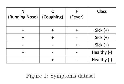
What is the predicted class for a person with running nose but no coughing, and no fever: sick, or healthy? Use a Naive Bayes classifier.
The predicted class is Healthy(-).
If p_+ and p_- are the numerators of the Naive Bayes comparison that represent a Sick(+) prediction and a Healthy(-) prediction, respectively, we have to compare: \begin{aligned} p_+=P(N,\bar C,\bar F|+)P(+)\quad \text{and}\quad p_-=P(N,\bar C,\bar F|-)P(-). \end{aligned}
We can find: \begin{aligned} &P(+)=\frac35\\ &P(-)=\frac25 \\ &P(N,\bar C,\bar F|+)=P(N|+)P(\bar C|+)P(\bar F|+)=\frac23\times \frac13\times\frac13=\frac{2}{27}\\ &P(N,\bar C,\bar F|-)=P(N|-)P(\bar C|-)P(\bar F|-)=\frac12\times \frac12\times 1=\frac{1}{4}. \end{aligned}
Then we can build up our comparison: \begin{aligned} p_+&= P(+)P(N,\bar C,\bar F|+) = \frac35\times\frac{2}{27}=\frac{2}{45}\quad \\ p_-&= P(-)P(N,\bar C,\bar F|-) = \frac25\times\frac{1}{4}=\frac{1}{10}\\ p_-&>p_+ \end{aligned}
So, the predicted class is Healthy(-).
What is the predicted class for a person with a running nose and fever, but no coughing? Use a Naive Bayes classifier.
The predicted class is Sick(+).
From the dataset we see P(F|-)=0, so we know: P(N,\bar C, F|-)=P(N|-)P(\bar C|-)P(F|-)=0
This will make p_- = P(N,\bar C, F|-)P(-) = 0
Contrast this against P(F|+), P(N|+), and P(\bar C|+), which are all nonzero values, making P(N,\bar C, F|+), (and therefore p_+) nonzero.
So p_+>p_-. This means our predicted class is Sick(+).
To deal with cases of unseen features, we used “smoothing" in class. If we use the”smoothing" method discussed in class, then what is the probability of a person having running nose and fever, but no coughing if that person was diagnosed “healthy"?
With smoothing, the result is \dfrac{1}{16}.
To apply smoothing, we add 1 to the numerator, and add the number of possible categories of the given event, healthiness (which would be 2 possible options in this case: sick, or healthy) to the denominator of our conditional probabilities. That way, other probabilities avoid being multiplied by zero. Let’s smooth our three conditional probabilities:
P(N|-)= \frac{1}{2} \to \frac{1 + 1}{2 + 2} = \frac{2}{4} P(\bar C|-)= \frac{1}{2} \to \frac{1 + 1}{2 + 2} = \frac{2}{4}
P(F|-)=0 is a zero probability that also needs to be smoothed. The smoothed version becomes: P(F|-)= \frac{0}{2} \to \frac{0 + 1}{2 + 2} = \frac{1}{4}
We carry on evaluating P(N,\bar C, F|-), just as the problem asks.
\begin{aligned} P(N,\bar C, F|-)=P(N|-)P(\bar C|-)P(F|-)=\frac24\times \frac24\times \frac14=\frac{1}{16}. \end{aligned}
In part (a), what are the odds of a person being “sick" who has running nose but no coughing, and no fever? (Hint: the formula for the odds of an event A is \text{odds}(A) = \frac{P(A)}{1 - P(A)})
\text{Odds of being sick}=\frac27
Using previous information, we have that the probability of a person being sick with a running nose but no coughing and no fever is:
\begin{aligned} P(+|N,\bar C,\bar F)=\frac{p_+}{P(N,\bar C,\bar F)}=\frac{\frac{2}{45}}{\frac{1}{5}}=\frac29. \end{aligned}
\begin{aligned} \text{Odds of being sick}=\frac{P(+|N,\bar C,\bar F)}{1-P(+|N,\bar C,\bar F)}=\frac27. \end{aligned}
Say someone fit a logistic regression model to a dataset containing n points (x_1,y_1),(x_2,y_2),\cdots,(x_n,y_n) where x_is are features and y_i\in\{-1,+1\} are labels. The estimated parameters are w_0,~w_1, that is, given feature x, the predicted probability of belonging to class y=+1 is
\begin{aligned} P(y=+1|x)=\frac{1}{1+\exp(-w_0-w_1x)}. \end{aligned}
Interpret the meaning of w_1=1.
One interpretation is as follows:
“If x is increased by 1, then the odds of y=+1 increases by a factor of \exp(1)=2.718.”