← return to practice.dsc40a.com
Instructor(s): Janine Tiefenbruck
This exam was administered in person. Students had 50 minutes to take this exam.
Source: Spring 2023 Final Part 1, Problem 1
For a given dataset \{y_1, y_2, \dots, y_n\}, let M_{abs}(h) represent the median absolute error of the constant prediction h on that dataset (as opposed to the mean absolute error R_{abs}(h)).
For the dataset \{4, 9, 10, 14, 15\}, what is M_{abs}(9)?
5
The first step is to calculate the absolute errors (|y_i - h|).
\begin{align*} \text{Absolute Errors} &= \{|4-9|, |9-9|, |10-9|, |14-9|, |15-9|\} \\ \text{Absolute Errors} &= \{|-5|, |0|, |1|, |5|, |6|\} \\ \text{Absolute Errors} &= \{5, 0, 1, 5, 6\} \end{align*}
Now we have to order the values inside of the absolute errors: \{0, 1, 5, 5, 6\}. We can see the median is 5, so M_{abs}(9) =5.
For the same dataset \{4, 9, 10, 14, 15\}, find another integer h such that M_{abs}(9) = M_{abs}(h).
5 or 15
Our goal is to find another number that will give us the same median of absolute errors as in part (a).
One way to do this is to plug in a number and guess. Another way requires noticing you can modify 10 (the middle element) to become 5 in either direction (negative or positive) because of the absolute value.
We can solve this equation to get |10-x| = 5 \rightarrow x = 15 \text{ and } x = 5.
We can then test this by following the same steps as we did in part (a).
For x = 15: \begin{align*} \text{Absolute Errors} &= \{|4-15|, |9-15|, |10-15|, |14-15|, |15-15|\} \\ \text{Absolute Errors} &= \{|-11|, |-6|, |-5|, |-1|, |0|\} \\ \text{Absolute Errors} &= \{11, 6, 5, 1, 0\} \end{align*}
Then we order the elements to get the absolute errors: \{0, 1, 5, 6, 11\}. We can see the median is 5, so M_{abs}(15) =5.
For x = 5: \begin{align*} \text{Absolute Errors} &= \{|4-5|, |9-5|, |10-5|, |14-5|, |15-5|\} \\ \text{Absolute Errors} &= \{|-1|, |4|, |5|, |9|, |10|\} \\ \text{Absolute Errors} &= \{1, 4, 5, 9, 10\} \end{align*}
We do not have to re-order the elements because they are in order already. We can see the median is 5, so M_{abs}(5) =5.
Based on your answers to parts (a) and (b), discuss in at most two sentences what is problematic about using the median absolute error to make predictions.
The numbers 5 and 15 are clearly bad predictions (close to the extreme values in the dataset), yet they are considered just as good a prediction by this metric as the number 9, which is roughly in the center of the dataset. Intuitively, 9 is a much better prediction, but this way of measuring the quality of a prediction does not recognize that.
Source: Spring 2023 Final Part 1, Problem 2
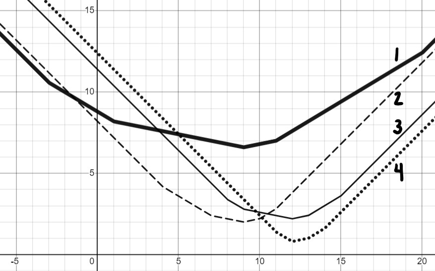
Match each dataset with the graph of its mean absolute error, R_{abs}(h).
\{4, 7, 9, 10, 11\}
Graph 1
Graph 2
Graph 3
Graph 4
Graph 2
The important thing to note here is the y axis is equal to R_{abs}(h) and the x axis is equal to our h. The easiest way to figure out which graph belongs to which dataset is to choose some numbers for h and see if a line matches up with the chosen points.
| h^* | R_{abs}(h) |
|---|---|
| 0 | \frac{1}{5}\sum_{i = 1}^{5}|y_i-0| = \frac{1}{5} \cdot 41 \approx 8 |
| 8 | \frac{1}{5}\sum_{i = 1}^{5}|y_i-8| = \frac{1}{5} \cdot 11 = 2 |
| 18 | \frac{1}{5}\sum_{i = 1}^{5}|y_i-18| = \frac{1}{5} \cdot 49 \approx 10 |
When looking at these three places we can see that this dataset matches Graph 2.
\{-3, 1, 9, 11, 20\}
Graph 1
Graph 2
Graph 3
Graph 4
Graph 1
We will use the same approach we used in part (a).
| h^* | R_{abs}(h) |
|---|---|
| 0 | \frac{1}{5}\sum_{i = 1}^{5}|y_i-0| = \frac{1}{5} \cdot 44 \approx 9 |
| 8 | \frac{1}{5}\sum_{i = 1}^{5}|y_i-8| = \frac{1}{5} \cdot 34 \approx 7 |
| 18 | \frac{1}{5}\sum_{i = 1}^{5}|y_i-18| = \frac{1}{5} \cdot 56 \approx 11 |
When looking at these three places we can see that this dataset matches Graph 1.
\{8, 9, 12, 13, 15\}
Graph 1
Graph 2
Graph 3
Graph 4
Graph 3
We will use the same approach we used in the previous parts.
| h^* | R_{abs}(h) |
|---|---|
| 0 | \frac{1}{5}\sum_{i = 1}^{5}|y_i-0| = \frac{1}{5} \cdot 44 \approx 11 |
| 8 | \frac{1}{5}\sum_{i = 1}^{5}|y_i-8| = \frac{1}{5} \cdot 17 \approx 3 |
| 18 | \frac{1}{5}\sum_{i = 1}^{5}|y_i-18| = \frac{1}{5} \cdot 33 \approx 7 |
When looking at these three places we can see that this dataset matches Graph 3.
\{11, 12, 12, 13, 14\}
Graph 1
Graph 2
Graph 3
Graph 4
Graph 4
We will use the same approach we used in the previous parts.
| h^* | R_{abs}(h) |
|---|---|
| 0 | \frac{1}{5}\sum_{i = 1}^{5}|y_i-0| = \frac{1}{5} \cdot 62 \approx 12 |
| 8 | \frac{1}{5}\sum_{i = 1}^{5}|y_i-8| = \frac{1}{5} \cdot 22 \approx 4 |
| 18 | \frac{1}{5}\sum_{i = 1}^{5}|y_i-18| = \frac{1}{5} \cdot 28 \approx 6 |
When looking at these three places we can see that this dataset
matches Graph 4. Another way would be choosing the only option not
chosen in the other parts yet!
Source: Spring 2023 Final Part 1, Problem 3
You and a friend independently perform gradient descent on the same function, but after 100 iterations, you have different results. Which of the following is sufficient on its own to explain the difference in your results? Note: When we say “same function” we assume the learning rate and initial predictions are the same too until said otherwise.
Select all that apply.
The function is nonconvex.
The function is not differentiable.
You and your friend chose different learning rates.
You and your friend chose different initial predictions.
None of the above.
Bubbles 3: “You and your friend chose different learning rates.”
If the function is nonconvex and you and your friend have the same initial prediction and learning rate you should end up in the same location local or global minimum.
If the function is not differentiable then you cannot perform gradient descent, so this cannot be an answer.
If you and your friend chose different learning rates it is possible to have different results because if you have a really large learning rate you might be hopping over the global minimum without properly converging. Your friend could choose a smaller learning rate, which will allow you to converge to the global minimum.
If you and your friend chose the same initial predictions you are guaranteed to end up in the same spot.
Because two of the option choices are possible the answer cannot be “None of the above.”
Source: Spring 2023 Final Part 1, Problem 4
In simple linear regression, our goal was to fit a prediction rule of the form H(x) = w_0 + w_1x. We found many equivalent formulas for the slope of the regression line:
w_1^* =\displaystyle\frac{\displaystyle\sum_{i=1}^n (x_i - \overline x)(y_i - \overline y)}{\displaystyle\sum_{i=1}^n (x_i - \overline x)^2} = \displaystyle\frac{\displaystyle\sum_{i=1}^n (x_i - \overline x)y_i}{\displaystyle\sum_{i=1}^n (x_i - \overline x)^2} = r \cdot \displaystyle\frac{\sigma_y}{\sigma_x}
Show that any one of the above formulas is equivalent to the formula below.
\displaystyle\frac{\displaystyle\sum_{i=1}^n (x_i - \overline x)(y_i + 2)}{\displaystyle\sum_{i=1}^n (x_i - \overline x)^2}
In other words, this is yet another formula for w_1^*.
We’ll show the equivalence to the middle formula above. Since the denominators are the same, we just need to show \begin{align*} \displaystyle\sum_{i=1}^n (x_i - \overline x)(y_i + 2) &= \displaystyle\sum_{i=1}^n (x_i - \overline x)y_i.\\ \displaystyle\sum_{i=1}^n (x_i - \overline x)(y_i + 2) &= \displaystyle\sum_{i=1}^n (x_i - \overline x)y_i + \displaystyle\sum_{i=1}^n (x_i - \overline x)\cdot2 \\ &= \displaystyle\sum_{i=1}^n (x_i - \overline x)y_i + 2\cdot\displaystyle\sum_{i=1}^n (x_i - \overline x) \\ &= \displaystyle\sum_{i=1}^n (x_i - \overline x)y_i + 2\cdot0 \\ &= \displaystyle\sum_{i=1}^n (x_i - \overline x)y_i\\ \end{align*}
This proof uses a fact we’ve already seen, that \displaystyle\sum_{i=1}^n (x_i - \overline x) = 0. It is not necesary to re-prove this fact when answering this question.
Source: Spring 2023 Final Part 1, Problem 5
Suppose we want to predict how long it takes to run a Jupyter notebook on Datahub. For 100 different Jupyter notebooks, we collect the following 5 pieces of information:
cells: number of cells in the notebook
lines: number of lines of code
max iterations: largest number of iterations in any loop in the notebook, or 1 if there are no loops
variables: number of variables defined in the notebook
runtime: number of seconds for the notebook to run on Datahub
Then we use multiple regression to fit a prediction rule of the form H(\text{cells, lines, max iterations, variables}) = w_0 + w_1 \cdot \text{cells} \cdot \text{lines} + w_2 \cdot (\text{max iterations})^{\text{variables} - 10}
What are the dimensions of the design matrix X?
\begin{bmatrix} & & & \\ & & & \\ & & & \\ \end{bmatrix}_{r \times c}
So, what should r and c be for: r rows \times c columns.
100 \text{ rows} \times 3 \text{ columns}
There should be 100 rows because there are 100 different Jupyter notebooks with different information within them. There should be 3 columns, one for each w_i. In this case we have w_0, which means X will have a column of ones, w_1, which means X will have a second column of \text{cells} \cdot \text{lines}, and w_2, which will be the last column in X containing \text{max iterations})^{\text{variables} - 10}.
In one sentence, what does the entry in row 3, column 2 of the design matrix X represent? (Count rows and columns starting at 1, not 0).
This entry represents the product of the number of cells and number of lines of code for the third Jupyter notebook in the training dataset.
Source: Spring 2023 Final Part 1, Problem 6
Now we solve the normal equations and find the solution to be \begin{aligned} \vec{w}^* &= \begin{bmatrix} w_0^* \\ w_1^* \\ w_2^* \end{bmatrix} \end{aligned} Define a new vector: \begin{aligned} \vec{w}^{\circ} &= \begin{bmatrix} w_0^{\circ} \\ w_1^{\circ} \\ w_2^{\circ} \end{bmatrix} = \begin{bmatrix} w_0^*+3 \\ w_1^*-4 \\ w_2^*-6 \end{bmatrix} \end{aligned}and consider the two prediction rules
\begin{aligned} H^*(\text{cells, lines, max iterations, variables}) &= w_0^* + w_1^* \cdot \text{cells} \cdot \text{lines} + w_2^* \cdot (\text{max iterations})^{\text{variables} - 10}\\ H^{\circ}(\text{cells, lines, max iterations, variables}) &= w_0^{\circ} + w_1^{\circ} \cdot \text{cells} \cdot \text{lines} + w_2^{\circ} \cdot (\text{max iterations})^{\text{variables} - 10} \end{aligned}Let \text{MSE} represent the mean squared error of a prediction rule, and let \text{MAE} represent the mean absolute error of a prediction rule. Select the symbol that should go in each blank.
\text{MSE}(H^*) ___ \text{MSE}(H^{\circ})
\leq
\geq
=
\leq
It is given that \vec{w}^* is the optimal parameter vector. Here’s one thing we know about the optimal parameter vector \vec{w}^*: it is optimal, which means that any changes made to it will, at best, keep our predictions of the exact same quality, and, at worst, reduce the quality of our predictions and increase our error. And since \vec{w} \degree is just the optimal parameter vector but with some small changes to the weights, it stands that \vec{w} \degree is liable to create equal or greater error!
In other words, \vec{w} \degree is a slightly worse version of \vec{w}^*, meaning that H \degree(x) is a slightly worse version of H^*(x). So, H \degree(x) will have equal or higher error than H^*(x).
Hence: \text{MSE}(H^*) \leq \text{MSE}(H^{\circ})