Let \vec{x} = \begin{bmatrix} x_1 \\ x_2
\end{bmatrix}. Consider the function g(\vec{x}) = x_1^2 + x_2^2 + x_1 x_2 - 4x_1 - 6x_2 +
8.
Problem 1.1
Find \nabla g(\vec{x}), the gradient
of g(\vec{x}), and use it to show that
\nabla g\left( \begin{bmatrix} 1 \\ 2
\end{bmatrix} \right) = \begin{bmatrix} 0 \\ -1
\end{bmatrix}.
To calculate the gradient, we take the partial derivatives of g with respect to both x_1 and x_2,
and arrange these partial derivatives as a vector. \frac{\partial g}{\partial x_1} = 2x_1 + x_2 -
4\frac{\partial g}{\partial x_2} =
2x_2 + x_1 - 6 Writing these as a vector, we obtain the gradient
above.
We’d like to find the vector \vec{x}^* that minimizes g(\vec{x}) using gradient descent. Perform
one iteration of gradient descent by hand, using the initial guess \vec{x}^{(0)} = \begin{bmatrix} 1 \\ 2
\end{bmatrix} and the learning rate \alpha = \frac{1}{4}. Show your work, and put
a \boxed{\text{box}} around your final
answer for \vec{x}^{(1)}.
Given some new function f(x) that is
convex, prove that the function g(x) = a f(x)
+ b is also convex, where a and
b are positive real constants.
Note: this function g(\cdot) is
entirely different from g(\vec{x}) on
the previous page.
Hint: Use the fact that we already know f(x) is convex and the formal definition of
convexity: for all t\in[0, 1], \ (1-t) f(c) +
t f(d) \geq f\left((1-t)c + td\right).
To show that g(x) is convex, we want
to begin with the expression (1-t) g(c) + t
g(d) and use algebra to show it’s \geq
g\left((1-t)c + td\right).
Let \vec{x} = \begin{bmatrix} x_1 \\ x_2
\end{bmatrix}. Consider the function g(\vec{x}) = (x_1 - 3)^2 + (x_1^2 -
x_2)^2.
Problem 2.1
Find \nabla g(\vec{x}), the gradient
of g(\vec{x}), and use it to show that
\nabla g\left( \begin{bmatrix} -1 \\ 1
\end{bmatrix} \right) = \begin{bmatrix} -8 \\ 0
\end{bmatrix}.
We’d like to find the vector \vec{x}^* that minimizes g(\vec{x}) using gradient descent. Perform
one iteration of gradient descent by hand, using the initial guess \vec{x}^{(0)} = \begin{bmatrix} -1 \\ 1
\end{bmatrix} and the learning rate \alpha = \frac{1}{2}. In other words, what is
\vec{x}^{(1)}?
Consider the function f(t) = (t - 3)^2 +
(t^2 - 1)^2. Select the true statement below.
f(t) is convex and has a global
minimum.
f(t) is not convex, but has a global
minimum.
f(t) is convex, but doesn’t have a
global minimum.
f(t) is not convex and doesn’t have
a global minimum.
f(t) is not convex, but has a global
minimum.
It is seen that f(t) isn’t convex,
which can be verified using the second derivative test: f'(t) = 2(t - 3) + 2(t^2 - 1) 2t = 2t - 6 +
4t^3 - 4t = 4t^3 - 2t - 6f''(t) = 12t^2 - 2
Clearly, f''(t) < 0 for
many values of t (e.g. t = 0), so f(t) is not always convex.
However, f(t) does have a global
minimum – its output is never less than 0. This is because it can be
expressed as the sum of two squares, (t -
3)^2 and (t^2 - 1)^2,
respectively, both of which are greater than or equal to 0.
You and a friend independently perform gradient descent on the same
function, but after 100 iterations, you have different results. Which of
the following is sufficient on its own to explain the
difference in your results? Note: When we say “same
function” we assume the learning rate and initial predictions are the
same too until said otherwise.
Select all that apply.
The function is nonconvex.
The function is not differentiable.
You and your friend chose different learning rates.
You and your friend chose different initial predictions.
None of the above.
Bubbles 3: “You and your friend chose different learning rates.”
If the function is nonconvex and you and your friend have the same
initial prediction and learning rate you should end up in the same
location local or global minimum.
If the function is not differentiable then you cannot perform
gradient descent, so this cannot be an answer.
If you and your friend chose different learning rates it is possible
to have different results because if you have a really large learning
rate you might be hopping over the global minimum without properly
converging. Your friend could choose a smaller learning rate, which will
allow you to converge to the global minimum.
If you and your friend chose the same initial predictions you are
guaranteed to end up in the same spot.
Because two of the option choices are possible the answer cannot be
“None of the above.”
Consider the function R(h) = \sqrt{(h -
3)^2 + 1} = ((h - 3)^2 + 1)^{\frac{1}{2}}, which is a convex and
differentiable function with only one local minimum.
Problem 4.1
Perform by hand two iterations of the gradient descent algorithm on
this function, using an initial prediction of h_0 = 2 and a learning rate of \alpha = 2\sqrt{2}. Show your work and your
final answers, h_1 and h_2.
h_1 = 4, h_2 = 2
The updating rule for gradient descent in the one-dimensional case
is: h_{i+1} = h_{i} - \alpha \cdot
\frac{dR}{dh}(h_i)
We can find \frac{dR}{dh} by taking
the derivative of R(h): \frac{d}{dh}R(h) = \frac{d}{dh}(\sqrt{(h - 3)^2 +
1}) = \dfrac{h-3}{\sqrt{\left(h-3\right)^2+1}}
Now we can use \alpha = 2\sqrt{2}
and h_0 = 2 to begin updating:
With more iterations, will we eventually converge to the minimizer?
Explain.
No, this algorithm will not converge to the minimizer because if we
do more iterations, we’ll keep oscillating back and forth between
predictions of 2 and 4. We showed the first two iterations of the
algorithm in part 1, but the next two would be exactly the same, and the
two after that, and so on. This happens because the learning rate is too
big, resulting in steps that are too big, and we keep jumping over the
true minimizer at h = 3.
In general, the logarithm of a convex function is not convex. Give an
example of a function f(x) such that
f(x) is convex, but \log_{10}(f(x)) is not convex.
There are many correct answers to this question. Some simple answers
are f(x) = x and f(x) = x^2. The logarithms of these function
are \log_{10}(x) and 2\log_{10}(x), both of which are nonconvex
because there are pairs of points such that the line connecting them
goes below the function.
Remember to show your work and justify your answers.
Suppose we want to minimize the function
R(h) = e^{(h + 1)^2}
Problem 6.1
Without using gradient descent or calculus, what is the value h^* that minimizes R(h)?
h^* = -1
The minimum possible value of the exponent is 0, since anything squared is non-negative.
The exponent is 0 when (x+1)^2 = 0,
i.e. when x = -1. Since e^{(x+1)^2} gets larger as (x+1)^2 gets larger, the minimizing input
h^* is -1.
Problem 6.2
Now, suppose we want to use gradient descent to minimize R(h). Assume we use an initial guess of h_0 = 0. What is h_1? Give your answer in terms of a generic
step size, \alpha, and other constants.
(e is a constant.)
In our case, \frac{dR}{dh}(0) = 2(0 + 1)
e^{(0+1)^2} = 2e, so
h_1 = -\alpha \cdot 2e
Problem 6.3
Using your answers from the previous two parts, what should we set
the value of \alpha to be if we want to
ensure that gradient descent finds h^*
after just one iteration?
\alpha = \frac{1}{2e}
We know from the part (b) that h_1 =
-\alpha \cdot 2e, and we know from part (a) that h^* = -1. If gradient descent converges in
one iteration, that means that h_1 =
h^*; solving this yields
-\alpha \cdot 2e = -1 \implies \alpha =
\frac{1}{2e}
Problem 6.4
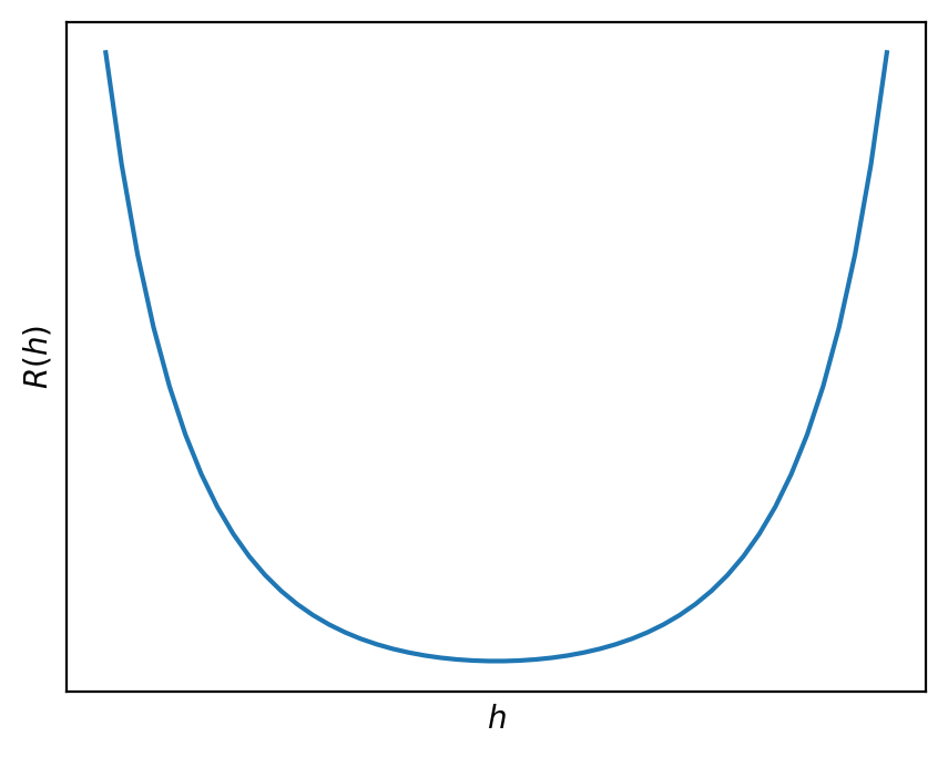
Below is a graph of R(h) with no
axis labels.
True or False: Given an appropriate choice of step size, \alpha, gradient descent is guaranteed to
find the minimizer of R(h).
True.
R(h) is convex, since the graph is
bowl shaped. (It can also be proved that R(h) is convex using the second derivative
test.) It is also differentiable, as we saw in part (b). As a result,
since it’s both convex and differentiable, gradient descent is
guaranteed to be able to minimize it given an appropriate choice of step
size.
Suppose that we are given f(x) = x^3 +
x^2 and learning rate \alpha =
1/4.
Problem 7.1
Write down the updating rule for gradient descent in general, then
write down the updating rule for gradient descent for the function f(x).
In general, the updating rule for gradient descent is: x_{i + 1} = x_i - \alpha \nabla f(x_i) = x_i -
\alpha \frac{\partial f}{\partial x}(x_i), where \alpha \in \mathbb{R}_+ is the learning rate
or step size. For this function, since f is a single-variable function, we can write
down the updating rule as: x_{i + 1} = x_i -
\alpha \frac{df}{dx}(x_i) = x_i - \alpha f'(x_i). We also
have: \frac{df}{dx} = f'(x) = 3x^2 +
2x, thus the updating rule can be written down as: x_{i + 1} = x_i - \alpha(3x_i^2 + 2x_i) =
-\frac{3}{4} x_i^2 + \frac{1}{2}x_i.
Problem 7.2
If we start at x_0 = -1, should we
go left or right? Can you verify this mathematically? What is x_1? Can gradient descent converge? If so,
where it might converge to, given appropriate step size?
We have f'(x_0) = f'(-1) = 3(-1)^2
+ 2(-1) = 1 > 0, so we go left, and x_1 = x_0 - \alpha f'(x_0) = -1 - \frac{1}{4} =
-\frac{5}{4}. Intuitively, the gradient descent cannot
converge in this case because \text{lim}_{x \rightarrow -\infty} f(x) =
-\infty,
We need to find all local minimums and local maximums. First, we
solve the equation f'(x) = 0 to
find all critical points.
We have: f'(x) = 0 \Leftrightarrow
3x^2 + 2x = 0 \Leftrightarrow x = -\frac{2}{3} \ \ \text{and} \ \ x =
0.
Now, we consider the second-order derivative: f''(x) = \frac{d^2f}{dx^2} = 6x +
2.
We have f''(x) = 0 only when
x = -1/3. Thus, for x < -1/3, f''(x) is negative or the slope f'(x) decreases; and for x > -1/3, f''(x) is positive or the slope f'(x) increases. Keep in mind that -1 < -2/3 < -1/3 < 0 < 1.
Therefore, f has a local maximum at
x = -2/3 and a local minimum at x = 0. If the gradient descent starts at
x_0 = -1 and it always goes left then
it will never meet the local minimum at x =
0, and it will go left infinitely. We say the gradient descent
cannot converge, or is divergent.
Problem 7.3
If we start at x_0 = 1, should we go
left or right? Can you verify this mathematically? What is x_1? Can gradient descent converge? If so,
where it might converge to, given appropriate step size?
We have f'(x_0) = f'(-1) = 3 \cdot
1^2 + 2 \cdot 1 = 5 > 0, so we go left, and
x_1 = x_0 - \alpha f'(x_0) = 1 -
\frac{1}{4} \cdot 5 = -\frac{1}{4}.
From the previous part, function f
has a local minimum at x = 0, so the
gradient descent can converge (given appropriate step
size) at this local minimum.
Problem 7.4
Write down 1 condition to terminate
the gradient descent algorithm (in general).
There are several ways to terminate the gradient descent
algorithm:
If the change in the optimization objective is too small, i.e.
|f(x_i) - f(x_{i + 1})| < \epsilon
where \epsilon is a small
constant,
If the gradient is close to zero or the norm of the gradient is
very small, i.e. \|\nabla f(x_i)\| <
\lambda where \lambda is a small
constant.
Let f(x):\mathbb{R}\to\mathbb{R} be a
convex function. f(x) is not
necessarily differentiable. Use the definition of convexity to prove the
following:
\begin{aligned}
2f(2) \leq f(1)+f(3)
\end{aligned}
Here is the definition of convexity:
f(tx_{1}+(1-t)x_{2})\leq
tf(x_{1})+(1-t)f(x_{2})
Since f(x) is a convex function, we
know that this inequality is satisfied for all choices of x_1 and x_2
on the real number line and all choices of t
\in [0, 1]. This problem boils down to finding a choice of x_1, x_2,
and t to morph the definition of
convexity into our desired inequality.
One such successful combination is x_1=1, x_2=3, and t=0.5. This makes tx_{1}+(1-t)x_{2}=0.5\cdot 1 + (1 - 0.5)\cdot
3=2. Therefore: f(tx_{1}+(1-t)x_{2})=f(2) \leq
0.5f(x_{1})+f(x_{2})=0.5 (f(1)+f(3))2f(2) \leq f(1)+f(3).
The strategy for these variable choices boils down to trying to make
the left side of the definition of convexity “look more” like the left
side of our desired inequality, and trying to make the right side of the
definition of convexity “look more” like the right side of our desired
inequality.
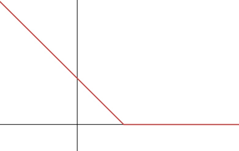
Let (x,y) be a sample where x is the feature and y denotes the class. Consider the following
loss function, known as Hinge loss, for a predictor z of y:
\begin{aligned}
L(z)=\max(0,1-yz).
\end{aligned}
For all the following questions assume y=1.
Problem 9.1
Plot L(z).
The plot should have a y-intercept at (0,1) with slope of -1 until (1,0), where it plateaus to zero.
Problem 9.2
Consider the following smoothed version of Hinge loss.
\begin{aligned}
L_s(z)=\begin{cases}
0 & \text{ if } z\geq 1\\
\frac12(1-z)^2 & \text{ if } 0<z< 1\\
0.5-z & \text{ if } z\leq 0
\end{cases}.
\end{aligned}
Is the global minima of L_s(z)
unique?
The minima is not unique since the minimum value is 0 and any z\geq 1 achieves L(z)=0.
Problem 9.3
Perform two steps of gradient descent with step size \alpha=1 for L_s(z) starting from the point z_0=-0.5.
For z_0=-0.5, our point lies on the
linear part of the function (L_s(z)=0.5-z), therefore {L'}_s(z)=-1. Our update is then: z_1=z_0 - \alpha
{L'}_s(z_0)=-0.5+1=0.5
For z_1=0.5, our point lies on the
quadratic part of the function (L_s(z)=0.5(1-z)^2), therefore {L'}_s(z)=-(1-z). The update is then
z_2=z_1 - \alpha
{L'}_s(z_1)=0.5+(1-0.5)=1
You and a friend independently perform gradient descent on the same
function, but after 200 iterations, you
have different results. Which of the following is sufficient on
its own to explain the difference in your results?
Note: When we say “same function” we assume the
learning rate and initial predictions are the same too until said
otherwise.
Select all that apply.
The function is nonconvex.
The function is not differentiable.
You and your friend chose different learning rates.
You and your friend chose the same initial predictions.
None of the above.
Bubbles 3: “You and your friend chose different learning rates.”
If the function is nonconvex and you and your friend have the same
initial prediction and learning rate you should end up in the same
location local or global minimum.
If the function is not differentiable then you cannot perform
gradient descent, so this cannot be an answer.
If you and your friend chose different learning rates it is possible
to have different results because if you have a really large learning
rate you might be hopping over the global minimum without properly
converging. Your friend could choose a smaller learning rate, which will
allow you to converge to the global minimum.
If you and your friend chose the same initial predictions you are
guaranteed to end up in the same spot.
Because two of the option choices are possible the answer cannot be
“None of the above.”
Suppose there is a dataset contains four values: -2, -1,
2, 4.
You would like to use gradient descent to minimize the mean square error
over this dataset.
Problem 11.1
Write down the expression of mean square error and its derivative
given this dataset.
R_{sq}(h) =
\dfrac{1}{4}\sum_{i=1}^{4}(y_i-h)^2
Recall the equation for R_{sq}(h) =
\frac{1}{n}\sum_{i=1}^{n}(y_i-h)^2, so we simply need to replace
n with 4 because there are 4 elements in our dataset.
Since we have the equation for R_{sq}(h) we can calculate the
derivative:
\begin{align*}
\frac{dR_{sq}(h)}{dh} &=
\frac{dR_{sq}(h)}{dh}(\frac{1}{4}\sum_{i=1}^{4}(y_i-h)^2) \\
&= \frac{1}{4}\sum_{i=1}^{4}\frac{dR_{sq}(h)}{dh}((y_i-h)^2) \\
\end{align*}
We can use the chain rule to find the derivative of (y_i-h)^2. Recall the chain rule is: \frac{df(x)}{dx}[(f(x))^n] = n(f(x))^{n-1} \cdot
f'(x).
Suppose you choose the initial position to be h_0 and the learning rate to be \frac{1}{4}. After two gradient descent
steps, h_2=\frac{1}{4}. What is the
value of h_0?
h_{0} = -\frac{5}{4}
The gradient descent equation is given by: \begin{aligned}
h_i = h_{i-1} - \alpha \frac{dR_{sq}(h_{i-1})}{dh}
\end{aligned} Recall the learning rate is equal to \alpha. We can plug in \alpha = \frac{1}{4}, h_2 = \frac{1}{4}, and i=2, in that case we obtain: \begin{aligned}
\frac{1}{4} &= h_{1} - \alpha \frac{dR_{sq}(h_{1})}{dh}\\
&= h_{1} - \alpha \frac{1}{2}\sum_{i=1}^{4}(h_1-y_i)\\
&= h_{1} - \frac{1}{8}(h_{1} + 2 + h_{1} + 1 + h_{1} - 2 +
h_{1} - 4)\\
&= h_{1} - \frac{1}{8}(4h_{1} -3)\\
\end{aligned} Solving this equation, we obtain that h_{1} = -\frac{1}{4}. We can then repeat this
step once more to obtain h_0: \begin{aligned}
-\frac{1}{4} &= h_{0} - \alpha \frac{dR_{sq}(h_{0})}{dh}\\
&= h_{0} - \frac{1}{4}(h_{0} + 2 + h_{0} + 1 + h_{0} - 2 +
h_{0} - 4)\\
&= h_{0} - \frac{1}{8}(4h_{0} -3)\\
\end{aligned} Solving this equation, we obtain that h_{0} = -\frac{5}{4}.
Problem 11.3
Given that we set the tolerance of gradient descent to be 0.1. How many additional
steps beyond h_2 do we need to
take to reach convergence?
0
1
2
3
4
It will never converge
2 or 3 additional steps (both are correct).
The gradient descent equation is given by: \begin{aligned}
h_i = h_{i-1} - \alpha \frac{dR_{sq}(h_{i-1})}{dh}
\end{aligned} Now we start from \alpha
= \frac{1}{4}, h_2 =
\frac{1}{4}, and i=2, in that
case we obtain: \begin{aligned}
h_{3} &= h_{2} - \alpha \frac{dR_{sq}(h_{2})}{dh}\\
&= h_{2} - \frac{1}{8}(4h_{2} -3)\\
&= \frac{1}{4} - \frac{1}{8}(1 -3)\\
&= \frac{1}{2}\\
\end{aligned} Iteratively, we have: \begin{aligned}
h_{4} &= h_{3} - \alpha \frac{dR_{sq}(h_{3})}{dh}\\
&= h_{3} - \frac{1}{8}(4h_{3} -3)\\
&= \frac{1}{2} - \frac{1}{8}(2 -3)\\
&= \frac{5}{8}\\
\end{aligned}\begin{aligned}
h_{5} &= h_{4} - \alpha \frac{dR_{sq}(h_{4})}{dh}\\
&= h_{3} - \frac{1}{8}(4h_{4} -3)\\
&= \frac{5}{8} - \frac{1}{8}(\frac{5}{2}-3)\\
&= \frac{11}{16}\\
\end{aligned} from h_4 to h_5, the change is smaller than the
tolerance. That means we need additional 2 or 3 steps
to reach convergence (depending on if you actually perform h_4 to h_5,
so both 2 and 3 are considered correct answer).
The hyperbolic cosine function is defined as cosh(x) = \frac{1}{2}(e^{x} + e^{-x}). In
this problem, we aim to prove the convexity of this function using power
series expansion.
Problem 12.1
Prove that f(x) = x^{n} is convex if
n is an even integer.
If n is even, then n-2 must also be even, therefore f''(x) = n(n-1)x^{n-2} will always be
a positive number. This means the second derivative of f(x) is always larger than 0 and therefore passes the second derivative
test.
Problem 12.2
Power series expansion is a powerful tool to analyze complicated
functions. In power series expansion, a function can be written as an
infinite sum of polynomial functions with certain coefficients. For
example, the exponential function can be written as: \begin{align*}
e^{x} = \sum_{n=0}^{\infty}\frac{x^{n}}{n!} = 1 + x +
\frac{x^{2}}{2} + \frac{x^{3}}{6} + \frac{x^{4}}{24} + ...
\end{align*}
where n! denotes the factorial of
n, defined as the product of all
positive integers up to n, i.e. n! = 1\cdot 2\cdot 3\cdot ... \cdot
(n-1)\cdot n. Given the power series expansion of e^{x} above, write the power series expansion
of e^{-x} and explicitly specify the
first 5 terms, i.e., similar to the format of the equation above.
Within this infinite sum, if n is even, then the negative sign in
(-x)^{n} will disappear; if n is odd,
then the negative sign in (-x)^{n} will
be kept and travel out of the parenthesis. Therefore we have:
Therefore, cosh(x)=\displaystyle\frac{e^{x}+e^{-x}}{2}
is a sum of x^{n}, where n is even. Since we have already proved in
part (a) that x^{n} are always convex
for even n, cosh(x) is an infinite sum of convex
functions and therefore also convex.
Let \vec{x} = \begin{bmatrix} x_1 \\ x_2
\end{bmatrix}. Consider the function g(\vec{x}) = (x_1 - 3)^2 + (x_1^2 -
x_2)^2.
Problem 13.1
Find \nabla g(\vec{x}), the gradient
of g(\vec{x}), and use it to show that
\nabla g\left( \begin{bmatrix} -1 \\ 1
\end{bmatrix} \right) = \begin{bmatrix} -8 \\ 0
\end{bmatrix}.
We’d like to find the vector \vec{x}^* that minimizes g(\vec{x}) using gradient descent. Perform
one iteration of gradient descent by hand, using the initial guess \vec{x}^{(0)} = \begin{bmatrix} -1 \\ 1
\end{bmatrix} and the learning rate \alpha = \frac{1}{2}. In other words, what is
\vec{x}^{(1)}?
Consider the function f(t) = (t - 3)^2 +
(t^2 - 1)^2. Select the true statement below.
f(t) is convex and has a global
minimum.
f(t) is not convex, but has a global
minimum.
f(t) is convex, but doesn’t have a
global minimum.
f(t) is not convex and doesn’t have
a global minimum.
f(t) is not convex, but has a global
minimum.
It is seen that f(t) isn’t convex,
which can be verified using the second derivative test: f'(t) = 2(t - 3) + 2(t^2 - 1) 2t = 2t - 6 +
4t^3 - 4t = 4t^3 - 2t - 6f''(t) = 12t^2 - 2
Clearly, f''(t) < 0 for
many values of t (e.g. t = 0), so f(t) is not always convex.
However, f(t) does have a global
minimum – its output is never less than 0. This is because it can be
expressed as the sum of two squares, (t -
3)^2 and (t^2 - 1)^2,
respectively, both of which are greater than or equal to 0.
👋
Feedback: Find an error? Still confused? Have a suggestion?
Let us know
here.