← return to practice.dsc40a.com
This page contains all problems about Simple Linear Regression.
Source: Spring 2024 Final, Problem 3
Suppose we’re given a dataset of n points, (x_1, y_1), (x_2, y_2), ..., (x_n, y_n), where \bar{x} is the mean of x_1, x_2, ..., x_n and \bar{y} is the mean of y_1, y_2, ..., y_n.
Using this dataset, we create a transformed dataset of n points, (x_1', y_1'), (x_2', y_2'), ..., (x_n', y_n'), where:
x_i' = 4x_i - 3 \qquad y_i' = y_i + 24
That is, the transformed dataset is of the form (4x_1 - 3, y_1 + 24), ..., (4x_n - 3, y_n + 24).
We decide to fit a simple linear hypothesis function H(x') = w_0 + w_1x' on the transformed dataset using squared loss. We find that w_0^* = 7 and w_1^* = 2, so H^*(x') = 7 + 2x'.
Suppose we were to fit a simple linear hypothesis function through the original dataset, (x_1, y_1), (x_2, y_2), ..., (x_n, y_n), again using squared loss. What would the optimal slope be?
2
4
6
8
11
12
24
8.
Relative to the dataset with x', the dataset with x has an x-variable that’s “compressed” by a factor of 4, so the slope increases by a factor of 4 to 2 \cdot 4 = 8.
Concretely, this can be shown by looking at the formula 2 = r\frac{SD(y')}{SD(x')}, recognizing that SD(y') = SD(y) since the y values have the same spread in both datasets, and that SD(x') = 4 SD(x).
Recall, the hypothesis function H^* was fit on the transformed dataset,
(x_1', y_1'), (x_2', y_2'), ..., (x_n', y_n'). H^* happens to pass through the point (\bar{x}, \bar{y}). What is the value of \bar{x}? Give your answer as an integer with no variables.
5.
The key idea is that the regression line always passes through (\text{mean } x, \text{mean } y) in the dataset we used to fit it. So, we know that: 2 \bar{x'} + 7 = \bar{y'}. This first equation can be rewritten as: 2 \cdot (4\bar{x} - 3) + 7 = \bar{y} + 24.
We’re also told this line passes through (\bar{x}, \bar{y}), which means that it’s also true that: 2 \bar{x} + 7 = \bar{y}.
Now we have a system of two equations:
\begin{cases} 2 \cdot (4\bar{x} - 3) + 7 = \bar{y} + 24 \\ 2 \bar{x} + 7 = \bar{y} \end{cases}
\dots and solving our system of two equations gives: \bar{x} = 5.
Source: Spring 2024 Final, Problem 5
Let \vec{x} = \begin{bmatrix} x_1 \\ x_2 \end{bmatrix}. Consider the function g(\vec{x}) = (x_1 - 3)^2 + (x_1^2 - x_2)^2.
Find \nabla g(\vec{x}), the gradient of g(\vec{x}), and use it to show that \nabla g\left( \begin{bmatrix} -1 \\ 1 \end{bmatrix} \right) = \begin{bmatrix} -8 \\ 0 \end{bmatrix}.
\nabla g(\vec{x}) = \begin{bmatrix} 2x_1 -6 + 4x_1(4x_1^2 - x_2) \\ -2(x_1^2 - x_2) \end{bmatrix}
We can find \nabla g(\vec{x}) by finding the partial derivatives of g(\vec{x}):
\frac{\partial g}{\partial x_1} = 2(x_1 - 3) + 2(x_1^2 - x_2)(2 x_1) \frac{\partial g}{\partial x_2} = 2(x_1^2 - x_2)(-1) \nabla g(\vec{x}) = \begin{bmatrix} 2(x_1 - 3) + 2(x_1^2 - x_2)(2 x_1) \\ 2(x_1^2 - x_2)(-1) \end{bmatrix} \nabla g\left(\begin{bmatrix} - 1 \\ 1 \end{bmatrix}\right) = \begin{bmatrix} 2(-1 - 4) + 2((-1)^2 - 1)(2(-1)) \\ 2((-1)^2 - 1) \end{bmatrix} = \begin{bmatrix} -8 \\ 0 \end{bmatrix}.
We’d like to find the vector \vec{x}^* that minimizes g(\vec{x}) using gradient descent. Perform one iteration of gradient descent by hand, using the initial guess \vec{x}^{(0)} = \begin{bmatrix} -1 \\ 1 \end{bmatrix} and the learning rate \alpha = \frac{1}{2}. In other words, what is \vec{x}^{(1)}?
\vec x^{(1)} = \begin{bmatrix} 3 \\ 1 \end{bmatrix}
Here’s the general form of gradient descent: \vec x^{(1)} = \vec{x}^{(0)} - \alpha \nabla g(\vec{x}^{(0)})
We can substitute \alpha = \frac{1}{2} and x^{(0)} = \begin{bmatrix} -1 \\ 1 \end{bmatrix} to get: \vec x^{(1)} = \begin{bmatrix} -1 \\ 1 \end{bmatrix} - \frac{1}{2} \nabla g(\vec x ^{(0)}) \vec x^{(1)} = \begin{bmatrix} -1 \\ 1 \end{bmatrix} - \frac{1}{2} \begin{bmatrix} -8 \\ 0 \end{bmatrix}
\vec{x}^{(1)} = \begin{bmatrix} -1 \\ 1 \end{bmatrix} - \frac{1}{2} \begin{bmatrix} -8 \\ 0 \end{bmatrix} = \begin{bmatrix} 3 \\ 1 \end{bmatrix}
Consider the function f(t) = (t - 3)^2 + (t^2 - 1)^2. Select the true statement below.
f(t) is convex and has a global minimum.
f(t) is not convex, but has a global minimum.
f(t) is convex, but doesn’t have a global minimum.
f(t) is not convex and doesn’t have a global minimum.
f(t) is not convex, but has a global minimum.
It is seen that f(t) isn’t convex, which can be verified using the second derivative test: f'(t) = 2(t - 3) + 2(t^2 - 1) 2t = 2t - 6 + 4t^3 - 4t = 4t^3 - 2t - 6 f''(t) = 12t^2 - 2
Clearly, f''(t) < 0 for many values of t (e.g. t = 0), so f(t) is not always convex.
However, f(t) does have a global minimum – its output is never less than 0. This is because it can be expressed as the sum of two squares, (t - 3)^2 and (t^2 - 1)^2, respectively, both of which are greater than or equal to 0.
Source: Fall 2022 Midterm, Problem 3
Mahdi runs a local pastry shop near UCSD and sells traditional desert called Baklava. He bakes Baklavas every morning to keep his promise of providing fresh Baklavas to his customers daily. Here is the amount of Baklava he sold each day during last week in pounds(lb): y_1=100, y_2=110, y_3=75, y_4=90, y_5=105, y_6=90, y_7=25
Mahdi needs your help as a data scientist to suggest the best constant prediction (h^*) of daily sales that minimizes the empirical risk using L(h,y) as the loss function. Answer the following questions and give a brief justification for each part. This problem has many parts, if you get stuck, move on and come back later!
Let L(h,y)=|y-h|. What is h^*? (We’ll later refer to this prediction as h_1^*).
As we have seen in lectures, the median minimizes the absolute loss risk function. h^*_1=\text{Median}(y_1, \cdots, y_7).
Let L(h,y)=(y-h)^2. What is h^*? (We’ll later refer to this prediction as h_2^*).
As we have seen in lectures, the mean minimizes the square loss risk function. h^*_2=\text{Mean}(y_1, \cdots, y_7).
True or False: Removing y_1 and y_3 from the dataset does not change h_2^*.
True
False
False. It changes the mean from 85 to 84. (However, the median is not changed.)
Mahdi thinks that y_7 is an outlier. Hence, he asks you to remove y_7 and update your predictions in parts (a) and (b) accordingly. Without calculating the new predictions, can you justify which prediction changes more? h^*_1 or h_2^*?
Removing y_7 affects h_2^* more than h_1^*. This is because the mean squared loss is more sensitive to outliers than absolute loss, and removing data changes the mean more.
True or False: Let L(y,h)=|y-h|^3. You can use the Gradient descent algorithm to find h^*.
True
False
False. The function |y-h|^3 is not differentiable everywhere so we can not use the gradient descent to find the minimum.
True or False: Let L(y,h)=\sin(y-h). The Gradient descent
algorithm is guaranteed to converge, provided that a proper learning
rate is given.
True
False
False. The function is not convex, so the gradient descent algorithm is not guaranteed to converge.
Mahdi has noticed that Baklava daily sale is associated with weather temperature. So he asks you to incorporate this feature to get a better prediction. Suppose the last week’s daily temperatures are x_1, x_2, \cdots, x_7 in Fahrenheit (F). We know that \bar x=65, \sigma_x=8.5 and the best linear prediction that minimizes the mean squared error is H^*(x)=-3x+w_0^*.
What is the correlation coefficient (r) between x and y? What does that mean?
r=-0.95. This means the weather temperature inversely affects Baklava sales, i.e., they are highly negatively correlated.
We know w_1^* = \frac{\sigma_y}{\sigma_x}r. We know that \sigma_x=8.5 and w_1^*=-3. We can find \sigma_y as follows:
\begin{aligned} \sigma_y^2 =& \frac{1}{n} \sum_{i = 1}^n (y_i - \bar{y})^2\\ =& \frac{1}{7}[(100-85)^2+(110-85)^2+(75-85)^2+(90-85)^2+(105-85)^2+(90-85)^2+(25-85)^2]\\ =&\frac{1}{7}[15^2+25^2+10^2+5^2+20^2+5^2+60^2]=714.28 \end{aligned}
Then, \sigma_y=26.7 which results in r=-0.95.
True or False: The unit of r is \frac{lb}{F} (Pound per Fahrenheit).
True
False
False. The correlation coefficient has no unit. (It is always a unitless number in [-1,1] range.)
Find w^*_0. (Hint: You’ll need to find \bar y for the given dataset)
w_0^*=280
Note that H(\bar x)=\bar y. Therefore, \begin{aligned} H(65)=-3\cdot 65 +w_0^*=85 \xrightarrow[]{}w_0^*=280. \end{aligned}
What would the best linear prediction H^*(x) be if we multiply all x_i’s by 2?
H^*(x) = -1.5x + 280
The standard deviation scales by a factor of 2, i.e., \sigma_x'=2\cdot \sigma_x.
The same
is true for the mean, i.e., \bar{x}'=2
\cdot \bar{x}.
The correlation r, standard deviation of the y-values \sigma_y, and the mean of the y-values \bar y do not change.
(You can verify
these claims by plugging 2x in for
x in their respective formulas and
seeing what happens, but it’s faster to visually reason why
this happens.)
Therefore, w_1'^*=\frac{\sigma_y'}{\sigma_x'}r' = \frac{(\sigma_y)}{(2\cdot\sigma_x)}(r) = \frac{w_1^*}{2} = -1.5.
We can find w_0'^* as follows:
\begin{align*} \bar{y}'&=H(\bar{x}')\\&=\frac{w_1^*}{2}(2\bar{x})+w_0'^*\\&=w_1^*\bar{x}+w_0'^* \\ &\downarrow \\ (85) &= -3(65) + w_0'^* \\ w_0'^*&=280 \end{align*}
So, H^*(x) would be -1.5x + 280.
What would the best linear prediction H^*(x) be if we add 20 to all x_i’s?
H^*(x) = -3x + 340
All parameters remain unchanged except \bar{x}'=\bar{x}+20. Since r, \sigma_x and \sigma_y are not changed, w_1^* does not change. Then, one can find w_0^* as follows:
\begin{align*} \bar{y}'&=H(\bar{x}') \\ &\downarrow \\ (85) &=-3(65+20)+w_0^* \\ w_0^*&=340 \end{align*}
So, H^*(x) would be -3x + 340.
Source: Fall 2021 Final Exam, Problem 5
Suppose we have a dataset of n houses that were recently sold in the San Diego area. For each house, we have its square footage and most recent sale price. The correlation between square footage and price is r.
First, we minimize mean squared error to fit a linear prediction rule that uses square footage to predict price. The resulting prediction rule has an intercept of w_0^* and slope of w_1^*. In other words,
\text{predicted price} = w_0^* + w_1^* \cdot \text{square footage}
We’re now interested in minimizing mean squared error to fit a linear prediction rule that uses price to predict square footage. Suppose this new regression line has an intercept of \beta_0^* and slope of \beta_1^*.
What is \beta_1^*? Give your answer in terms of one or more of n, r, w_0^*, and w_1^*. Show your work.
\beta_1^* = \frac{r^2}{w_1^*}
Throughout this solution, let x represent square footage and y represent price.
We know that w_1^* = r \frac{\sigma_y}{\sigma_x}. But what about \beta_1^*?
When we take a rule that predicts price from square footage and transform it into a rule that predicts square footage from price, the roles of x and y have swapped; suddenly, square footage is no longer our independent variable, but our dependent variable, and vice versa for price. This means that the altered dataset we work with when using our new prediction rule has \sigma_x standard deviation for its dependent variable (square footage), and \sigma_y for its independent variable (price). So, we can write the formula for \beta_1^* as follows: \beta_1^* = r \frac{\sigma_x}{\sigma_y}
In essence, swapping the independent and dependent variables of a dataset changes the slope of the regression line from r \frac{\sigma_y}{\sigma_x} to r \frac{\sigma_x}{\sigma_y}.
From here, we can use a little algebra to get our \beta_1^* in terms of one or more n, r, w_0^*, and w_1^*:
\begin{align*} \beta_1^* &= r \frac{\sigma_x}{\sigma_y} \\ w_1^* \cdot \beta_1^* &= w_1^* \cdot r \frac{\sigma_x}{\sigma_y} \\ w_1^* \cdot \beta_1^* &= ( r \frac{\sigma_y}{\sigma_x}) \cdot r \frac{\sigma_x}{\sigma_y} \end{align*}
The fractions \frac{\sigma_y}{\sigma_x} and \frac{\sigma_x}{\sigma_y} cancel out and we get:
\begin{align*} w_1^* \cdot \beta_1^* &= r^2 \\ \beta_1^* &= \frac{r^2}{w_1^*} \end{align*}
For this part only, assume that the following quantities hold:
Given this information, what is \beta_0^*? Give your answer as a constant, rounded to two decimal places. Show your work.
\beta_0^* = 1278.56
We start with the formula for the intercept of the regression line. Note that x and y are opposite what they’d normally be since we’re using price to predict square footage.
\beta_0^* = \bar{x} - \beta_1^* \bar{y}
We’re told that the average square footage of homes in the dataset is 2000, so \bar{x} = 2000. We also know from part (a) that \beta_1^* = \frac{r^2}{w_1^*}, and from the information given in this part this is \beta_1^* = \frac{r^2}{w_1^*} = \frac{0.6^2}{250}.
Finally, we need the average price of all homes in the dataset, \bar{y}. We aren’t given this information directly, but we can use the fact that (\bar{x}, \bar{y}) are on the regression line that uses square footage to predict price to find \bar{y}. Specifically, we have that \bar{y} = w_0^* + w_1^* \bar{x}; we know that w_0^* = 1000, \bar{x} = 2000, and w_1^* = 250, so \bar{y} = 1000 + 2000 \cdot 250 = 501000.
Putting these pieces together, we have
\begin{align*} \beta_0^* &= \bar{x} - \beta_1^* \bar{y} \\ &= 2000 - \frac{0.6^2}{250} \cdot 501000 \\ &= 2000 - 0.6^2 \cdot 2004 \\ &= 1278.56 \end{align*}
Source: Fall 2021 Midterm, Problem 4
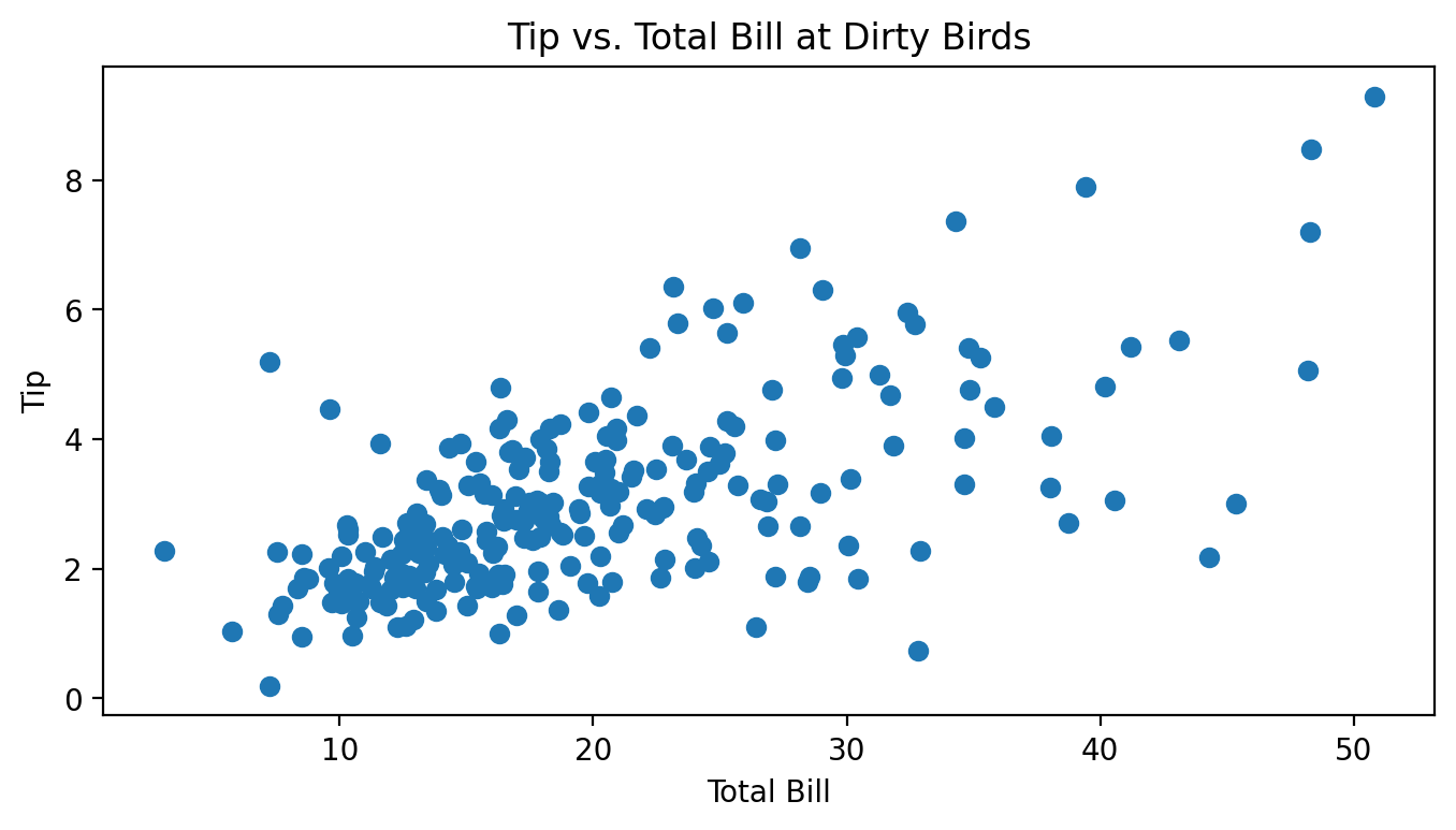
Billy, the avocado farmer from Homework 3, wasn’t making enough money growing avocados and decided to take on a part-time job as a waiter at the restaurant Dirty Birds on campus. For two months, he kept track of all of the total bills he gave out to customers along with the tips they then gave him, all in dollars. Below is a scatter plot of Billy’s tips and total bills.
Throughout this question, assume we are trying to fit a linear prediction rule H(x) = w_0 + w_1x that uses total bills to predict tips, and assume we are finding optimal parameters by minimizing mean squared error.
Which of these is the most likely value for r, the correlation between total bill and tips? Why?
-1 \qquad -0.75 \qquad -0.25 \qquad 0 \qquad 0.25 \qquad 0.75 \qquad 1
0.75.
It seems like there is a pretty strong, but not perfect, linear association between total bills and tips.
The variance of the tip amounts is 2.1. Let M be the mean squared error of the best linear prediction rule on this dataset (under squared loss). Is M less than, equal to, or greater than 2.1? How can you tell?
M is less than 2.1. The variance is equal to the MSE of the constant prediction rule.
Note that the MSE of the best linear prediction rule will always be less than or equal to the MSE of the best constant prediction rule h. The only case in which these two MSEs are the same is when the best linear prediction rule is a flat line with slope 0, which is the same as a constant prediction. In all other cases, the linear prediction rule will make better predictions and hence have a lower MSE than the constant prediction rule.
In this case, the best linear prediction rule is clearly not flat, so M < 2.1.
Suppose we use the formulas from class on Billy’s dataset and calculate the optimal slope w_1^* and intercept w_0^* for this prediction rule.
Suppose we add the value of 1 to every total bill x, effectively shifting the scatter plot 1 unit to the right. Note that doing this does not change the value of w_1^*. What amount should we add to each tip y so that the value of w_0^* also does not change? Your answer should involve one or more of \bar{x}, \bar{y}, w_0^*, w_1^*, and any constants.
Note: To receive full points, you must provide a rigorous explanation, though this explanation only takes a few lines. However, we will award partial credit to solutions with the correct answer, and it’s possible to arrive at the correct answer by drawing a picture and thinking intuitively about what happens.
We should add w_1^* to each tip y.
First, we present the rigorous solution.
Let \bar{x}_\text{old} represent the previous mean of the x’s and \bar{x}_\text{new} represent the new mean of the x’s. Then, we know that \bar{x}_\text{new} = \bar{x}_\text{old} + 1.
Also, let \bar{y}_\text{old} and \bar{y}_\text{new} represent the old and new mean of the y’s. We will try and find a relationship between these two quantities.
We want the two intercepts to be the same. The intercept for the old line is \bar{y}_\text{old} - w_1^* \bar{x}_\text{old} and the intercept for the new line is \bar{y}_\text{new} - w_1^* \bar{x}_\text{new}. Setting these equal yields
\begin{aligned} \bar{y}_\text{new} - w_1^* \bar{x}_\text{new} &= \bar{y}_\text{old} - w_1^* \bar{x}_\text{old} \\ \bar{y}_\text{new} - w_1^* (\bar{x}_\text{old} + 1) &= \bar{y}_\text{old} - w_1^* \bar{x}_\text{old} \\ \bar{y}_\text{new} &= \bar{y}_\text{old} - w_1^* \bar{x}_\text{old} + w_1^* (\bar{x}_\text{old} + 1) \\ \bar{y}_{\text{new}} &= \bar{y}_\text{old} + w_1^* \end{aligned}
Thus, in order for the intercepts to be equal, we need the mean of the new y’s to be w_1^* greater than the mean of the old y’s. Since we’re told we’re adding the same constant to each y that constant is w_1^*.
Another way to approach the question is as follows: consider any point that lies directly on a line with slope w_1^* and intercept w_0^*. Consider how the slope between two points on a line is calculated: \text{slope} = \frac{y_2 - y_1}{x_2 - x_1}. If x_2 - x_1 = 1, in order for the slope to remain fixed we must have that y_2 - y_1 = \text{slope}. For a concrete example, think of the line y = 5x + 2. The point (1, 7) is on the line, as is the point (1 + 1, 7 + 5) = (2, 12).
In our case, none of our points are guaranteed to be on the line defined by slope w_1^* and intercept w_0^*. Instead, we just want to be guaranteed that the points have the same regression line after being shifted. If we follow the same principle, though, and add 1 to every x and w_1^* to every y, the points’ relative positions to the line will not change (i.e. the vertical distance from each point to the line will not change), and so that will remain the line with the lowest MSE, and hence w_0^* and w_1^* won’t change.
Source: Fall 2022 Midterm, Problem 2
Calculate w_1^* and w_0^* of the linear regression line for the following dataset, \mathcal{D}. You may use the fill-in-the-blanks and the table below to organize your work.
\mathcal{D} = \{(0, 0), (4, 2), (5, 1)\}.
\bar x = \phantom{\hspace{.5in}} \bar y = \phantom{\hspace{.5in}}
| x_i | y_i | (x_i - \bar x) | (y_i - \bar y) | (x_i - \bar x)(y_i - \bar y) | (x_i - \bar x)^2 |
|---|---|---|---|---|---|
| 0 | 0 | ||||
| 4 | 2 | ||||
| 5 | 1 |
w_1^* =
w_0^* =
Finally, what can we say about the correlation r and the slope for this dataset (mathematically)?
\bar{x} = \frac{1}{3}(0 + 4 + 5) = 3
\quad \quad\bar{y} = \frac{1}{3}(0 + 2 + 1) =
1
| x_i | y_i | (x_i - \bar x) | (y_i - \bar y) | (x_i - \bar x)(y_i - \bar y) | (x_i - \bar x)^2 |
|---|---|---|---|---|---|
| 0 | 0 | -3 | -1 | 3 | 9 |
| 4 | 2 | 1 | 1 | 1 | 1 |
| 5 | 1 | 2 | 0 | 0 | 4 |
w_1^* = \displaystyle
\frac{\sum_{i=1}^n (x_i - \bar{x})(y_i - \bar{y})}{\sum_{i=1}^n (x_i -
\bar{x})^2}
= \frac{3 + 1 + 0}{9 + 1 + 4} = \frac{4}{14} = \frac{2}{7}
w_0^* = \bar{y} - w_1^* \bar{x} = 1 - \frac{2}{7} \cdot 3 = 1 - \frac{6}{7} = \frac{1}{7}
Because w_1^* = r \frac{\sigma_y}{\sigma_x} where the standard deviations \sigma_y and \sigma_x are non-negative, and w_1^* = 2/7 > 0, the correlation r is positive and the slope is positive.
Source: Fall 2022 Midterm, Problem 3
Mahdi runs a local pastry shop near UCSD and sells traditional desert called Baklava. He bakes Baklavas every morning to keep his promise of providing fresh Baklavas to his customers daily. Here is the amount of Baklava he sold each day during last week in pounds(lb): y_1=100, y_2=110, y_3=75, y_4=90, y_5=105, y_6=90, y_7=25
Mahdi needs your help as a data scientist to suggest the best constant prediction (h^*) of daily sales that minimizes the empirical risk using L(h,y) as the loss function. Answer the following questions and give a brief justification for each part. This problem has many parts, if you get stuck, move on and come back later!
Let L(h,y)=|y-h|. What is h^*? (We’ll later refer to this prediction as h_1^*).
As we have seen in lectures, the median minimizes the absolute loss risk function. h^*_1=\text{Median}(y_1, \cdots, y_7).
Let L(h,y)=(y-h)^2. What is h^*? (We’ll later refer to this prediction as h_2^*).
As we have seen in lectures, the mean minimizes the square loss risk function. h^*_2=\text{Mean}(y_1, \cdots, y_7).
True or False: Removing y_1 and y_3 from the dataset does not change h_2^*.
True
False
False. It changes the mean from 85 to 84. (However, the median is not changed.)
Mahdi thinks that y_7 is an outlier. Hence, he asks you to remove y_7 and update your predictions in parts (a) and (b) accordingly. Without calculating the new predictions, can you justify which prediction changes more? h^*_1 or h_2^*?
Removing y_7 affects h_2^* more than h_1^*. This is because the mean squared loss is more sensitive to outliers than absolute loss, and removing data changes the mean more.
True or False: Let L(y,h)=|y-h|^3. You can use the Gradient descent algorithm to find h^*.
True
False
False. The function |y-h|^3 is not differentiable everywhere so we can not use the gradient descent to find the minimum.
True or False: Let L(y,h)=\sin(y-h). The Gradient descent
algorithm is guaranteed to converge, provided that a proper learning
rate is given.
True
False
False. The function is not convex, so the gradient descent algorithm is not guaranteed to converge.
Mahdi has noticed that Baklava daily sale is associated with weather temperature. So he asks you to incorporate this feature to get a better prediction. Suppose the last week’s daily temperatures are x_1, x_2, \cdots, x_7 in Fahrenheit (F). We know that \bar x=65, \sigma_x=8.5 and the best linear prediction that minimizes the mean squared error is H^*(x)=-3x+w_0^*.
What is the correlation coefficient (r) between x and y? What does that mean?
r=-0.95. This means the weather temperature inversely affects Baklava sales, i.e., they are highly negatively correlated.
We know w_1^* = \frac{\sigma_y}{\sigma_x}r. We know that \sigma_x=8.5 and w_1^*=-3. We can find \sigma_y as follows:
\begin{aligned} \sigma_y^2 =& \frac{1}{n} \sum_{i = 1}^n (y_i - \bar{y})^2\\ =& \frac{1}{7}[(100-85)^2+(110-85)^2+(75-85)^2+(90-85)^2+(105-85)^2+(90-85)^2+(25-85)^2]\\ =&\frac{1}{7}[15^2+25^2+10^2+5^2+20^2+5^2+60^2]=714.28 \end{aligned}
Then, \sigma_y=26.7 which results in r=-0.95.
True or False: The unit of r is \frac{lb}{F} (Pound per Fahrenheit).
True
False
False. The correlation coefficient has no unit. (It is always a unitless number in [-1,1] range.)
Find w^*_0. (Hint: You’ll need to find \bar y for the given dataset)
w_0^*=280
Note that H(\bar x)=\bar y. Therefore, \begin{aligned} H(65)=-3\cdot 65 +w_0^*=85 \xrightarrow[]{}w_0^*=280. \end{aligned}
What would the best linear prediction H^*(x) be if we multiply all x_i’s by 2?
H^*(x) = -1.5x + 280
The standard deviation scales by a factor of 2, i.e., \sigma_x'=2\cdot \sigma_x.
The same
is true for the mean, i.e., \bar{x}'=2
\cdot \bar{x}.
The correlation r, standard deviation of the y-values \sigma_y, and the mean of the y-values \bar y do not change.
(You can verify
these claims by plugging 2x in for
x in their respective formulas and
seeing what happens, but it’s faster to visually reason why
this happens.)
Therefore, w_1'^*=\frac{\sigma_y'}{\sigma_x'}r' = \frac{(\sigma_y)}{(2\cdot\sigma_x)}(r) = \frac{w_1^*}{2} = -1.5.
We can find w_0'^* as follows:
\begin{align*} \bar{y}'&=H(\bar{x}')\\&=\frac{w_1^*}{2}(2\bar{x})+w_0'^*\\&=w_1^*\bar{x}+w_0'^* \\ &\downarrow \\ (85) &= -3(65) + w_0'^* \\ w_0'^*&=280 \end{align*}
So, H^*(x) would be -1.5x + 280.
What would the best linear prediction H^*(x) be if we add 20 to all x_i’s?
H^*(x) = -3x + 340
All parameters remain unchanged except \bar{x}'=\bar{x}+20. Since r, \sigma_x and \sigma_y are not changed, w_1^* does not change. Then, one can find w_0^* as follows:
\begin{align*} \bar{y}'&=H(\bar{x}') \\ &\downarrow \\ (85) &=-3(65+20)+w_0^* \\ w_0^*&=340 \end{align*}
So, H^*(x) would be -3x + 340.
Source: Spring 2023 Midterm 1, Problem 4
Suppose we are given a dataset of points \{(x_1, y_1), (x_2, y_2), \dots, (x_n, y_n)\} and for some reason, we want to make predictions using a prediction rule of the form H(x) = 17 + w_1x.
Write down an expression for the mean squared error of a prediction rule of this form, as a function of the parameter w_1.
MSE(w_1) = \dfrac1n \displaystyle\sum_{i=1}^n (y_i - (17 + w_1x_i))^2
Minimize the function MSE(w_1) to find the parameter w_1^* which defines the optimal prediction rule H^*(x) = 17 + w_1^*x. Show all your work and explain your steps.
Fill in your final answer below:
w_1^* = \dfrac{\displaystyle\sum_{i=1}^n x_i(y_i - 17)}{\displaystyle\sum_{i=1}^n x_i^2}
To minimize a function of one variable, we need to take the derivative, set it equal to zero, and solve. \begin{aligned} MSE(w_1) &= \dfrac1n \displaystyle\sum_{i=1}^n (y_i - 17 - w_1x_i)^2 \\ MSE'(w_1) &= \dfrac1n \displaystyle\sum_{i=1}^n -2x_i(y_i - 17 - w_1x_i)) \qquad \text{using the chain rule} \\ 0 &= \dfrac1n \displaystyle\sum_{i=1}^n -2x_i(y_i - 17) + \dfrac1n \displaystyle\sum_{i=1}^n 2x_i^2w_1 \qquad \text{splitting up the sum} \\ 0 &= \displaystyle\sum_{i=1}^n -x_i(y_i - 17) + \displaystyle\sum_{i=1}^n x_i^2w_1 \qquad \text{multiplying through by } \frac{n}{2} \\ w_1 \displaystyle\sum_{i=1}^n x_i^2 &= \displaystyle\sum_{i=1}^n x_i(y_i - 17) \qquad \text{rearranging terms and pulling out } w_1 \\ w_1 & = \dfrac{\displaystyle\sum_{i=1}^n x_i(y_i - 17)}{\displaystyle\sum_{i=1}^n x_i^2} \end{aligned}
True or False: For an arbitrary dataset, the prediction rule H^*(x) = 17 + w_1^*x goes through the point (\bar x, \bar y).
True
False
False.
When we fit a prediction rule of the form H(x) = w_0+w_1x using simple linear regression, the formula for the intercept w_0 is designed to make sure the regression line passes through the point (\bar x, \bar y). Here, we don’t have the freedom to control our intercept, as it’s forced to be 17. This means we can’t guarantee that the prediction rule H^*(x) = 17 + w_1^*x goes through the point (\bar x, \bar y).
A simple example shows that this is the case. Consider the dataset (-2, 0) and (2, 0). The point (\bar x, \bar y) is the origin, but the prediction rule H^*(x) does not pass through the origin because it has an intercept of 17.
True or False: For an arbitrary dataset, the mean squared error associated with H^*(x) is greater than or equal to the mean squared error associated with the regression line.
True
False
True.
The regression line is the prediction rule of the form H(x) = w_0+w_1x with the smallest mean squared error (MSE). H^*(x) is one example of a prediction rule of that form so unless it happens to be the regression line itself, the regression line will have lower MSE because it was designed to have the lowest possible MSE. This means the MSE associated with H^*(x) is greater than or equal to the MSE associated with the regression line.
Source: Spring 2023 Final Part 1, Problem 4
In simple linear regression, our goal was to fit a prediction rule of the form H(x) = w_0 + w_1x. We found many equivalent formulas for the slope of the regression line:
w_1^* =\displaystyle\frac{\displaystyle\sum_{i=1}^n (x_i - \overline x)(y_i - \overline y)}{\displaystyle\sum_{i=1}^n (x_i - \overline x)^2} = \displaystyle\frac{\displaystyle\sum_{i=1}^n (x_i - \overline x)y_i}{\displaystyle\sum_{i=1}^n (x_i - \overline x)^2} = r \cdot \displaystyle\frac{\sigma_y}{\sigma_x}
Show that any one of the above formulas is equivalent to the formula below.
\displaystyle\frac{\displaystyle\sum_{i=1}^n (x_i - \overline x)(y_i + 2)}{\displaystyle\sum_{i=1}^n (x_i - \overline x)^2}
In other words, this is yet another formula for w_1^*.
We’ll show the equivalence to the middle formula above. Since the denominators are the same, we just need to show \begin{align*} \displaystyle\sum_{i=1}^n (x_i - \overline x)(y_i + 2) &= \displaystyle\sum_{i=1}^n (x_i - \overline x)y_i.\\ \displaystyle\sum_{i=1}^n (x_i - \overline x)(y_i + 2) &= \displaystyle\sum_{i=1}^n (x_i - \overline x)y_i + \displaystyle\sum_{i=1}^n (x_i - \overline x)\cdot2 \\ &= \displaystyle\sum_{i=1}^n (x_i - \overline x)y_i + 2\cdot\displaystyle\sum_{i=1}^n (x_i - \overline x) \\ &= \displaystyle\sum_{i=1}^n (x_i - \overline x)y_i + 2\cdot0 \\ &= \displaystyle\sum_{i=1}^n (x_i - \overline x)y_i\\ \end{align*}
This proof uses a fact we’ve already seen, that \displaystyle\sum_{i=1}^n (x_i - \overline x) = 0. It is not necesary to re-prove this fact when answering this question.
Source: Winter 2022 Midterm 1, Problem 3
Suppose you have a dataset \{(x_1, y_1), (x_2,y_2), \dots, (x_8, y_8)\} with n=8 ordered pairs such that the variance of \{x_1, x_2, \dots, x_8\} is 50. Let m be the slope of the regression line fit to this data.
Suppose now we fit a regression line to the dataset \{(x_1, y_2), (x_2,y_1), \dots, (x_8, y_8)\} where the first two y-values have been swapped. Let m' be the slope of this new regression line.
If x_1 = 3, y_1 =7, x_2=8, and y_2=2, what is the difference between the new slope and the old slope? That is, what is m' - m? The answer you get should be a number with no variables.
Hint: There are many equivalent formulas for the slope of the regression line. We recommend using the version of the formula without \overline{y}.
m' - m = \dfrac{1}{16}
Using the formula for the slope of the regression line, we have: \begin{aligned} m &= \frac{\sum_{i=1}^n (x_i - \overline x)y_i}{\sum_{i=1}^n (x_i - \overline x)^2}\\ &= \frac{\sum_{i=1}^n (x_i - \overline x)y_i}{n\cdot \sigma_x^2}\\ &= \frac{(3-\bar{x})\cdot 7 + (8 - \bar{x})\cdot 2 + \sum_{i=3}^n (x_i - \overline x)y_i}{8\cdot 50}. \\ \end{aligned}
Note that by switching the first two y-values, the terms in the sum from i=3 to n, the number of data points n, and the variance of the x-values are all unchanged.
So the slope becomes:
\begin{aligned} m' &= \frac{(3-\bar{x})\cdot 2 + (8 - \bar{x})\cdot 7 + \sum_{i=3}^n (x_i - \overline x)y_i}{8\cdot 50} \\ \end{aligned}
and the difference between these slopes is given by:
\begin{aligned} m'-m &= \frac{(3-\bar{x})\cdot 2 + (8 - \bar{x})\cdot 7 - ((3-\bar{x})\cdot 7 + (8 - \bar{x})\cdot 2)}{8\cdot 50}\\ &= \frac{(3-\bar{x})\cdot 2 + (8 - \bar{x})\cdot 7 - (3-\bar{x})\cdot 7 - (8 - \bar{x})\cdot 2}{8\cdot 50}\\ &= \frac{(3-\bar{x})\cdot (-5) + (8 - \bar{x})\cdot 5}{8\cdot 50}\\ &= \frac{ -15+5\bar{x} + 40 -5\bar{x}}{8\cdot 50}\\ &= \frac{ 25}{8\cdot 50}\\ &= \frac{ 1}{16} \end{aligned}
Source: Winter 2024 Final Part 1, Problem 4
Albert collected 400 data points from a radiation detector. Each data point contains 3 features: feature A, feature B and feature C. The true particle energy E is also reported. Albert wants to design a linear regression algorithm to predict the energy E of each particle, given a combination of one or more of feature A, B, and C. As the first step, Albert calculated the correlation coefficients among A, B, C and E. He wrote it down in the following table, where each cell of the table represents the correlaton of two terms:
| A | B | C | E | |
|---|---|---|---|---|
| A | 1 | -0.99 | 0.13 | 0.8 |
| B | -0.99 | 1 | 0.25 | -0.95 |
| C | 0.13 | 0.25 | 1 | 0.72 |
| E | 0.8 | -0.95 | 0.72 | 1 |
Albert wants to start with a simple model: fitting only a single feature to obtain the true energy (i.e. y = w_0+w_1 x). Which feature should he choose as x to get the lowest mean square error?
A
B
C
B
B is the correct answer, because it has the highest absolute correlation (0.95), the negative sign in front of B just means it is negatively correlated to energy, and it can be compensated by a negative sign in the weight.
Albert wants to add another feature to his linear regression in part (a) to further boost the model’s performance. (i.e. y = w_0 + w_1 x + w_2 x_2) Which feature should he choose as x_2 to make additional improvements?
A
B
C
C
C is the correct answer, because although A has a higher correlation with energy, it also has an extremely high correlation with B (-0.99), that means adding A into the fit will not be too useful, since it provides almost the same information as B.
Albert further refines his algorithm by fitting a prediction rule of the form: \begin{aligned} H(A,B,C) = w_0 + w_1 \cdot A\cdot C + w_2 \cdot B^{C-7} \end{aligned}
Given this prediction rule, what are the dimensions of the design matrix X?
\begin{bmatrix} & & & \\ & & & \\ & & & \\ \end{bmatrix}_{r \times c}
So, what are r and c in r \text{ rows} \times c \text{ columns}?
400 \text{ rows} \times 3 \text{ columns}
Recall there are 400 data points, which means there will be 400 rows. There will be 3 columns; one is the bias column of all 1s, one is for the feature A\cdot C, and one is for the feature B^{C-7}.
Source: Winter 2024 Midterm 1, Problem 4
Note that we have two simplified closed form expressions for the estimated slope w in simple linear regression that you have already seen in discussions and lectures:
\begin{align*} w &= \frac{\sum_i (x_i - \overline{x}) y_i}{\sum_i (x_i - \overline{x})^2} \\ \\ w &= \frac{\sum_i (y_i - \overline{y}) x_i }{\sum_i (x_i - \overline{x})^2} \end{align*}
where we have dataset D = [(x_1,y_1), \ldots, (x_n,y_n)] and sample means \overline{x} = {1 \over n} \sum_{i} x_i, \quad \overline{y} = {1 \over n} \sum_{i} y_i. Without further explanation, \sum_i means \sum_{i=1}^n
Are (1) and (2) equivalent? That is, is the following equality true? Prove or disprove it. \sum_i (x_i - \overline{x}) y_i = \sum_i (y_i - \overline{y}) x_i
True. \begin{align*} & \sum_i (x_i - \overline{x}) y_i = \sum_i (y_i - \overline{y}) x_i \\ & \Leftrightarrow \sum_i x_i y_i - \overline{x} \sum_i y_i = \sum_i x_i y_i - \overline{y} \sum_i x_i \\ & \Leftrightarrow \overline{x} \sum_i y_i = \overline{y} \sum_i x_i \\ & \Leftrightarrow {1 \over n} \sum_i x_i \sum_i y_i = {1 \over n} \sum_i y_i \sum_i x_i \\ \end{align*}
True or False: If the dataset shifted right by a constant distance a, that is, we have the new dataset D_a = (x_1 + a,y_1), \ldots, (x_n + a,y_n), then will the estimated slope w change or not?
True
False
False. By (1) in part (a), we can view w as only being affected by x_i - \overline{x}, which is unchanged after shifting horizontally. Therefore, w is unchanged.
True or False: If the dataset shifted up by a constant distance b, that is, we have the new dataset D_b = [(x_1,y_1 + b), \ldots, (x_n,y_n + b)], then will the estimated slope w change or not?
True
False
False. By (2) in part (a), we can view w as only being affected by y_i - \overline{y}, which is unchanged after shifting vertically. Therefore, w is unchanged.
Source: Spring 2024 Final, Problem 3
Suppose we’re given a dataset of n points, (x_1, y_1), (x_2, y_2), ..., (x_n, y_n), where \bar{x} is the mean of x_1, x_2, ..., x_n and \bar{y} is the mean of y_1, y_2, ..., y_n.
Using this dataset, we create a transformed dataset of n points, (x_1', y_1'), (x_2', y_2'), ..., (x_n', y_n'), where:
x_i' = 4x_i - 3 \qquad y_i' = y_i + 24
That is, the transformed dataset is of the form (4x_1 - 3, y_1 + 24), ..., (4x_n - 3, y_n + 24).
We decide to fit a simple linear hypothesis function H(x') = w_0 + w_1x' on the transformed dataset using squared loss. We find that w_0^* = 7 and w_1^* = 2, so H^*(x') = 7 + 2x'.
Suppose we were to fit a simple linear hypothesis function through the original dataset, (x_1, y_1), (x_2, y_2), ..., (x_n, y_n), again using squared loss. What would the optimal slope be?
2
4
6
8
11
12
24
8.
Relative to the dataset with x', the dataset with x has an x-variable that’s “compressed” by a factor of 4, so the slope increases by a factor of 4 to 2 \cdot 4 = 8.
Concretely, this can be shown by looking at the formula 2 = r\frac{SD(y')}{SD(x')}, recognizing that SD(y') = SD(y) since the y values have the same spread in both datasets, and that SD(x') = 4 SD(x).
Recall, the hypothesis function H^* was fit on the transformed dataset,
(x_1', y_1'), (x_2', y_2'), ..., (x_n', y_n'). H^* happens to pass through the point (\bar{x}, \bar{y}). What is the value of \bar{x}? Give your answer as an integer with no variables.
5.
The key idea is that the regression line always passes through (\text{mean } x, \text{mean } y) in the dataset we used to fit it. So, we know that: 2 \bar{x'} + 7 = \bar{y'}. This first equation can be rewritten as: 2 \cdot (4\bar{x} - 3) + 7 = \bar{y} + 24.
We’re also told this line passes through (\bar{x}, \bar{y}), which means that it’s also true that: 2 \bar{x} + 7 = \bar{y}.
Now we have a system of two equations:
\begin{cases} 2 \cdot (4\bar{x} - 3) + 7 = \bar{y} + 24 \\ 2 \bar{x} + 7 = \bar{y} \end{cases}
\dots and solving our system of two equations gives: \bar{x} = 5.
Source: Summer Session 1 2025 Midterm, Problem 1
Let \{(x_i,y_i)\}_{i=1}^n be a dataset of scalar input-output pairs, and consider the simple linear regression model
f(a, b;\, x) = ax + b,\qquad a, b\in\mathbb{R}.
Let \gamma > 0 be a fixed constant which is understood to be separate from the training data and the weights. Define the \gamma-risk according to the formula
R_{\gamma}(a, b) = \gamma a^2 + \frac{1}{n}\sum_{i=1}^{n} (y_i - (ax_i + b))^2.
Find closed-form expressions for the global minimizers a^\ast, b^\ast of the \gamma-risk for the training data \{(x_i,y_i)\}_{i=1}^n. In your solution, you should clearly label and explain each step.
Source: Summer Session 1 2025 Midterm, Problem 5a-c
Let \{(x_i,y_i)\}_{i=1}^n be a dataset of scalar input-output pairs.
Suppose we model y using a simple linear regression model of the form
f(\vec{\theta};\, x) = \vec{\theta}^{(0)} + \vec{\theta}^{(1)}x, \qquad\vec{\theta}\in\mathbb{R}^2.
Prove that the line of best fit (with respect to MSE) passes through the point (\overline{x}, \overline{y}).
Suppose we model y using a simple polynomial regression model of the form
f(\vec{\theta};\, x) = \vec{\theta}^{(0)} + \vec{\theta}^{(1)}x+ \vec{\theta}^{(2)}x^2, \qquad\vec{\theta}\in\mathbb{R}^3.
Prove that the curve of best fit (with respect to MSE) passes through the point (\overline{x}, \overline{y} + \vec\theta^{\ast(2)}((\overline{x})^2 - \overline{x^2})), where
\overline{x^2} = \frac{1}{n}\sum_{i=1}^n x_i^2.
Using the same model as (b), suppose we minimize MSE and find optimal parameters \vec{\theta}^\ast. Further suppose we apply a shifting and scaling operation to the training targets, defining
\widetilde{y_i} = \alpha(y_i - \beta),\qquad\alpha,\beta\in\mathbb{R}.
Find formulas for the new optimal parameters, denoted \vec{\widetilde{\theta}}^\ast, in terms of the old parameters and \alpha, \beta.