← return to practice.dsc40a.com
Instructor(s): Gal Mishne
This exam was administered in person. They had a two sided 11in by 8.5in cheat sheet. Students had 50 minutes to take this exam.
For each statement below, fill in the circle indicating the word(s) or phrase(s) which would make the statement correct if added to the sentence. In several statements, (y_i)_{i=1}^n denotes a dataset of real numbers. You do not need to show your work for full credit, but partial credit may be awarded for supporting calculations and reasoning.
If x^\ast is a maximizer for f(x) and f(x)\geq 0 for all x, then x^\ast is a ________ for g(x)=3-f(x)^2.
\bigcirc minimizer \bigcirc maximizer \bigcirc neither
The correct answer is minimizer. Note that g(x) = 3-f(x)^2 is a monotone decreasing function for x\geq 0. Therefore, since f(x) \leq f(x^\ast) for all x, g(f(x)) \geq g(f(x^\ast)) for all x and this x^\ast is a minimizer for 3-f^2.
Suppose we wish to find a constant predictor for y using either squared or absolute loss. In high-stakes scenarios where outliers are rare but of great importance, it is better to use the ________ function.
\bigcirc absolute loss \bigcirc squared loss
The answer is squared loss, since it is more sensitive to outliers.
Let (1, 3, 4, 1, 2, -1) be a dataset of real numbers. The derivative of the empirical risk for the absolute loss L_{abs}(h) of a constant predictor h for the dataset is ________ when h=2.5.
\bigcirc positive \bigcirc negative \bigcirc zero
The derivative of empirical risk for absolute loss is given by R'(h) = \frac{1}{n}\sum_{i=1}^n\mathrm{sign}(h - y_i).
See lectures 3-4 for a derivation. Thus R'(2.5) = \frac{1}{6}(1 -1 -1 +1 +1 +1) = \frac{1}{3} > 0 .
So the correct answer is positive.
Alternative solution: Order the dataset: (-1,1, 1, 2, 3, 4 ). The loss is minimized in the range [1,2]. The point h=2.5 is to the right of this minimum and therefore the function is increasing at this point and the derivative must be positive.
Assume a dataset \{y_i\}_{i=1}^n satisfies y_i\in[0,1] for all i. Let h^\ast denote the optimal constant predictor for the dataset with respect to squared loss. Assume we sample a new data point y_{n+1} where y_{n+1}=y_4 - 2. Then the new minimizer h' is ________ the old minimizer h^\ast.
\bigcirc greater than \bigcirc less than \bigcirc equal to
We have that h^\ast is the mean of the original data, and h' is the mean of the new data. Therefore \begin{aligned} h' & = \frac{1}{n+1}\sum_{i=1}^{n+1}y_i = \frac{1}{n+1}(y_1+\cdots+y_n + (y_4 - 2)) \\ & = \frac{1}{n+1}(n h^\ast + (y_4 - 2)) \\ & = \frac{n}{n+1}h^\ast + \frac{y_4 - 2}{n+1} \end{aligned}
Note that y_4 - 2 \leq 1 - 2 = -1 < 0, so that \begin{aligned} \frac{n}{n+1}h^\ast + \frac{y_4 - 2}{n+1} < \frac{n}{n+1}h^\ast < h^\ast \end{aligned}
Therefore the correct answer is less than.
Let \epsilon > 0 be any positive real number. Define the smooth loss by the formula L_{\epsilon}(h, y_i) = \sqrt{|y_i - h|^2+ \epsilon^2}.
Then the optimal value of the empirical risk of L_{\epsilon} is ________ the optimal value of the empirical risk of the absolute loss function.
\bigcirc greater than \bigcirc less than \bigcirc equal to
Note that L_{\epsilon}(h, y_i) = \sqrt{|y_i - h|^2+ \epsilon^2} >\sqrt{|y_i - h|^2} = |y_i-h| = L_{abs}(h, y_i).
Therefore the minimum value of L_{\epsilon} is greater than the minimum value of L_{abs}.
[(12 points)] Suppose you are designing a central temperature control system for a network of n\geq 1 houses in a small town. Each house i has a preferred temperature y_i, and the importance of satisfying house i’s preference is represented by a weight a_i > 0, which represents the number of residents in each house.
The system is set to maintain a single uniform temperature h across all houses. To minimize dissatisfaction, you aim to minimize the weighted squared error:
R(h) = \frac{1}{n}\sum_{i=1}^n a_i (y_i - h)^2.
Find a formula for the optimal temperature h^\ast in terms of the various preferred temperatures y_1,\dotsc, y_n. Show all your calculations.
2in To minimize the function R(h) = \sum_{i=1}^n a_i (y_i - h)^2, we differentiate R(h) with respect to h and set the derivative equal to zero: \frac{dR(h)}{dh} = \frac{d}{dh} \sum_{i=1}^n a_i (y_i - h)^2 = -2 \sum_{i=1}^n a_i (y_i - h). Setting \frac{dR(h)}{dh} = 0, we get: \sum_{i=1}^n a_i y_i - \sum_{i=1}^n a_i h = 0. Simplifying: h \sum_{i=1}^n a_i = \sum_{i=1}^n a_i y_i. Solving for h^\ast: h^\ast = \frac{\sum_{i=1}^n a_i y_i}{\sum_{i=1}^n a_i}. Thus, the optimal temperature h^\ast is the weighted average of the preferred temperatures.
Suppose that the family which lives in house 1 has a baby, and their weight a_1 increases by one. Assuming their preferred temperature does not change, find an expression which relates the new optimal temperature h' to the old optimal temperature h^\ast you found in (a). Show all your calculations.
2in Let h' denote the new optimal temperature. The new weight for house 1 becomes a_1' = a_1 + 1. Using the formula for h^\ast, the new optimal temperature is: h' = \frac{(a_1 + 1)y_1 + \sum_{i=2}^n a_i y_i}{(a_1 + 1) + \sum_{i=2}^n a_i}. Expanding h': h' = \frac{a_1 y_1 + y_1 + \sum_{i=2}^n a_i y_i}{a_1 + 1 + \sum_{i=2}^n a_i}= \frac{ y_1 + \sum_{i=1}^n a_i y_i}{ 1 + \sum_{i=1}^n a_i}. Factoring out the original terms for h^\ast: h' = \frac{h^\ast \sum_{i=1}^n a_i + y_1}{\sum_{i=1}^n a_i + 1}. This relates the new optimal temperature h' to the original h^\ast by accounting for the additional weight and the corresponding preference.
You and your colleagues are discussing new and improved ways to set the weights used in the cost function. Your team comes up with three alternatives for setting the weights:
a_i = (\text{the number of residents in house $i$}),
b_i = 1 for all houses,
c_i = 1/(\text{the number of windows in house $i$}).
Assume each house is occupied by at least one person and has at least one window. Let
A denote the optimal risk of R(h) with respect to the weights a_i
B denote the optimal risk of R(h) with respect to the weights b_i
C denote the optimal risk of R(h) with respect to the weights c_i
Using the relations <,\leq,>,\geq,=, rank the numbers A,B,C from least to greatest. Explain your reasoning and don’t forget about the baby!
3in Note that for any choice of h, we have the following inequalities: \sum_{i=1}^n c_i (y_i - h)^2\leq \sum_{i=1}^n b_i (y_i - h)^2 <\sum_{i=1}^n a_i (y_i - h)^2. since c_i \leq 1 for all i, b_i = 1 for all i, and a_i\geq 1 for all i. Therefore the minimum values for each such function with respect to h will follow these inequalities. That is, C\leq B < A.
(Note we also accepted solution C\leq B \leq A for those who forgot about the baby ;) )
[(10 points)]
A local farmers’ market vendor sells homemade jam jars and is analyzing the relationship between the number of hours she spends at the market and the number of jam jars sold. Over three weekends, she collects the following data:
Weekend 1: Worked for 1 hour, sold 2 jars.
Weekend 2: Worked for 2 hours, sold 4 jars.
Weekend 3: Worked for 3 hours, sold 6 jars.
Noticing a perfect linear trend, she decides to model this relationship using linear regression. Let x_1 = 1, x_2=2, x_3=3 denote the number of hours she worked on the corresponding weekend and let y_1 = 2, y_2=4, y_3=6 denote the number of jars sold.
First, fill in the blanks in the table below which gathers relevant information for least squares regression. Then, find the optimal parameters w_0^\ast and w_1^\ast for a simple least squares linear model for her jar sales. Show all your calculations.
\begin{array}{|c|c|} \hline \text{Summation} & \text{Value} \\ \hline \sum_{i=1}^{3} x_i & 6 \\ \hline \sum_{i=1}^{3} y_i & \\ \hline \sum_{i=1}^{3} x_i y_i & 28 \\ \hline \sum_{i=1}^{3} x_i^2 & \\ \hline \end{array}
First, we calculate the missing values:
\sum_{i=1}^3 y_i = 2 + 4 + 6 = 12
\sum_{i=1}^3 x_i^2 = 1^2 + 2^2 + 3^2 = 1 + 4 + 9 = 14
The completed table is:
\begin{array}{|c|c|} \hline \text{Summation} & \text{Value} \\ \hline \sum_{i=1}^{3} x_i & 6 \\ \hline \sum_{i=1}^{3} y_i & 12 \\ \hline \sum_{i=1}^{3} x_i y_i & 28 \\ \hline \sum_{i=1}^{3} x_i^2 & 14 \\ \hline \end{array}
To calculate the optimal parameters, we use the least squares formulas:
w_1^* = \frac{\sum_{i=1}^3 x_iy_i - \frac{1}{3}\sum_{i=1}^3 x_i \sum_{i=1}^3 y_i}{\sum_{i=1}^3 x_i^2 - \frac{1}{3}\left(\sum_{i=1}^3 x_i\right)^2}
Substituting the values from our table:
w_1^* = \frac{28 - \frac{1}{3}(6 \cdot 12)}{14 - \frac{1}{3}(6^2)} = \frac{28 - 24}{14 - 12} = \frac{4}{2} = 2
Now we calculate w_0^*:
w_0^* = \frac{1}{3}\sum_{i=1}^3 y_i - w_1^* \cdot \frac{1}{3}\sum_{i=1}^3 x_i
Substituting values:
w_0^* = \frac{12}{3} - 2 \cdot \frac{6}{3} = 4 - 4 = 0
The optimal parameters are:
w_0^* = 0, \quad w_1^* = 2
This means the linear model is h(x) = 2x, which perfectly fits the data since each hour of work corresponds to exactly 2 jars sold.
On a fourth weekend, due to a festival, she couldn’t set up her stall but managed to sell 2 jars to early customers who contacted her directly. This data point is:
She now wants to understand how this outlier affects her overall analysis. Fill out the table below based on the new data point x_4 = 0, y_4=2 and then find the new optimal parameters w_0' and w_1' for a simple least squares linear model. Show all your calculations.
\begin{array}{|c|c|} \hline \text{Summation} & \text{Value} \\ \hline \sum_{i=1}^{4} x_i & \\ \hline \sum_{i=1}^{4} y_i & 14 \\ \hline \sum_{i=1}^{4} x_i y_i & 28 \\ \hline \sum_{i=1}^{4} x_i^2 & \\ \hline \end{array}
First, we fill in the table with the updated sums including the fourth data point:
\begin{array}{|c|c|} \hline \text{Summation} & \text{Value} \\ \hline \sum_{i=1}^{4} x_i & 6 \\ \hline \sum_{i=1}^{4} y_i & 14 \\ \hline \sum_{i=1}^{4} x_i y_i & 28 \\ \hline \sum_{i=1}^{4} x_i^2 & 14 \\ \hline \end{array}
Calculating the new slope w_1':
The formula for the optimal slope is:
w_1' = \frac{\sum_{i=1}^{4} x_i y_i - \frac{1}{4} \sum_{i=1}^{4} x_i \sum_{i=1}^{4} y_i}{\sum_{i=1}^{4} x_i^2 - \frac{1}{4} \left(\sum_{i=1}^{4} x_i\right)^2}
Substituting values:
w_1' = \frac{28 - \frac{1}{4}(6 \cdot 14)}{14 - \frac{1}{4}(6^2)} = \frac{28 - 21}{14 - 9} = \frac{7}{5} = 1.4
Calculating the new intercept w_0':
The formula for the optimal intercept is:
w_0' = \frac{1}{4} \sum_{i=1}^{4} y_i - w_1' \cdot \frac{1}{4} \sum_{i=1}^{4} x_i
Substituting values:
w_0' = \frac{14}{4} - 1.4 \cdot \frac{6}{4} = 3.5 - 2.1 = 1.4
Final Answer:
The new optimal parameters are:
w_0' = 1.4, \quad w_1' = 1.4
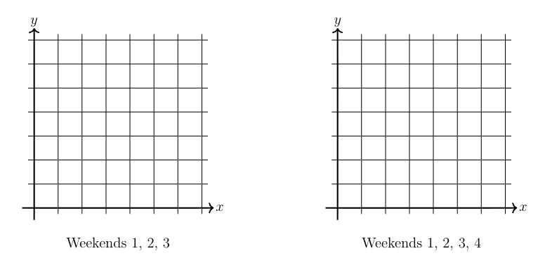
On each axis below draw: (i) the scatterplot of the corresponding data, and (ii) the line of best fit you found for the corresponding dataset in the preceding parts.
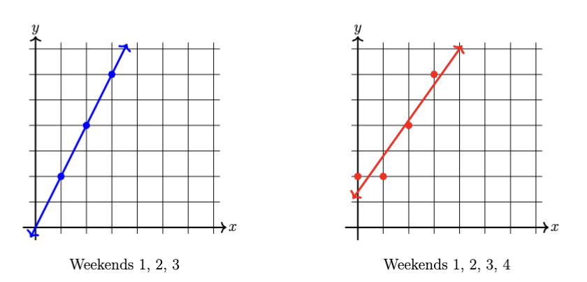
Based on the pictures in part (c), which dataset has greater mean squared error with respect to its optimal parameters? Why? You do not need to calculate the errors by hand to answer this question. Explain your reasoning.
The dataset with Weekends 1, 2, 3, and 4 will have a greater mean squared error. This is because the added outlier (Weekend 4) does not follow the original perfect linear trend and introduces a discrepancy between the data points and the new line of best fit
Consider the usual setup for a multiple regression problem, as follows. Let \vec{x}_1,\vec{x}_2,\dotsc, \vec{x}_{n}\in\mathbb{R}^d be a collection of feature vectors in \mathbb{R}^d, and let X\in\mathbb{R}^{n\times (d+1)} be the corresponding design matrix. Each \vec{x}_i has a label y_i\in\mathbb{R}, and let \vec{y}\in\mathbb{R}^n be the vector of labels. We wish to fit the data and labels with a linear model H(\vec{x}) = w_0 + w_1\vec{x}^{(1)} + w_2\vec{x}^{(2)}+\dotsc+ w_d\vec{x}^{(d)} \ = \vec{w}^T\mathrm{Aug}(\vec{x}). where \vec{w}\in\mathbb{R}^{d+1} is the vector of coefficients with intercept. Let \vec{w}^\ast denote the optimal parameter vector with respect to mean squared error.
For each statement below, fill in the circle indicating the word(s) or phrase(s) which would make the statement correct if added to the sentence. You do not need to show your work for full credit, but partial credit may be awarded for supporting calculations and reasoning.
At \vec{w}^\ast, the residual vector \vec{y}-X\vec{w}^\ast is ________ to the column space of the design matrix X.
\bigcirc neither \bigcirc orthogonal \bigcirc parallel
At \vec{w}^\ast, the residual vector \vec{y} - X\vec{w}^\ast is orthogonal to the column space of X. This is derived from the normal equations: X^T(\vec{y} - X\vec{w}^\ast) = 0, which imply that the residuals are perpendicular to the space spanned by the columns of X.
The optimal parameter vector w^\ast is found by setting the ________ of the mean squared error equal to ________ and solving the resulting equation.
\bigcirc (residuals, \vec{y}) \bigcirc (gradient, the zero vector) \bigcirc (predicted labels, X\vec{w})
The optimal parameter vector \vec{w}^\ast is found by setting the gradient of the mean squared error to the zero vector. The gradient is: \nabla_w \| \vec{y} - X\vec{w} \|^2 = -2X^T(\vec{y} - X\vec{w}), and solving X^T(X\vec{w} - \vec{y}) = 0 leads to the normal equation, which gives the minimum.
If the features in X are linearly ________, the matrix X^TX will be ________, making the normal equation solution possibly undefined.
\bigcirc (dependent, nonsingular) \bigcirc (independent, singular) \bigcirc (dependent, noninvertible)
If the features in X are linearly dependent, the matrix X^TX will be singular (noninvertible). Linear dependence implies that the columns of X are not linearly independent, leading to a determinant of zero for X^TX, which makes solving the normal equations impossible.
If \vec{c}\in\mathbb{R}^d is a fixed vector, and we define \vec{z}_i' = \vec{x}_i + \vec{c}, then the new optimal parameter vector \vec{w}' for the data \{\vec{z}_i\}_{i=1}^{n} and labels \vec{y} is equal to ________.
\bigcirc \vec{w}^\ast + \mathrm{Aug}(\vec{c}) \bigcirc \vec{w}^\ast \bigcirc \vec{w}^\ast except possibly for w_0
The new optimal parameter vector \vec{w}' is \vec{w}^\ast except possibly for w_0. Adding \vec{c} shifts the features, leaving w_1, w_2, \dots, w_d unchanged but altering the intercept: w_0' = w_0 - \vec{w}^T \vec{c}.
(Think of the simple linear regression model - if we shift all the x_i’s by constant c this doesn’t affect the slope w_1 but does affect the intercept w_0.)
For the remaining two parts, fill in the circle which contains the gradient of each function. You do not need to show your work for full credit, but partial credit may be awarded for supporting calculations and reasoning.
Calculate the gradient with respect to \vec{x} of F(\vec{x}) = \vec{w}^T\mathrm{Aug}(\vec{x}).
\bigcirc \begin{bmatrix} w_1 & w_2 & \dotsc & w_d \end{bmatrix}^T \bigcirc \vec{x} \bigcirc \begin{bmatrix} w_0 & w_1 & \dotsc & w_d \end{bmatrix}^T
The gradient of F(\vec{x}) = \vec{w}^T\mathrm{Aug}(\vec{x}) with respect to \vec{x} is \begin{bmatrix} w_1 & w_2 & \dotsc & w_d \end{bmatrix}^T. The first slot in \mathrm{Aug}(\vec{x}) is a constant 1, which cancels out when differentiating.
Calculate the gradient with respect to \vec{w} of F(\vec{w}) = \|\vec{y}-X\vec{w}\|^2.
\bigcirc -2X^TX\vec{w} \bigcirc -2(\vec{y}-X\vec{w}) \bigcirc -2X^T(\vec{y}-X\vec{w})
First expand the squared norm: F(\vec{w}) = (\vec{y} - X\vec{w})^T (\vec{y} - X\vec{w})
The gradient of F(\vec{w}) with respect to \vec{w} is: \nabla_{\vec{w}} F(\vec{w}) = \nabla_{\vec{w}} \left[ \vec{y}^T\vec{y} - 2\vec{y}^T X\vec{w} + \vec{w}^T X^T X \vec{w} \right]
Since \vec{y}^T\vec{y} does not depend on \vec{w}, its derivative is zero. The derivative of -2\vec{y}^T X\vec{w} is: \nabla_{\vec{w}} \left( -2\vec{y}^T X\vec{w} \right) = -2 X^T \vec{y}
The derivative of \vec{w}^T X^T X \vec{w} is (HW4 Problem 2): \nabla_{\vec{w}} \left( \vec{w}^T X^T X \vec{w} \right) = 2 X^T X \vec{w}
Combine the derivatives: \nabla_{\vec{w}} F(\vec{w}) = -2 X^T \vec{y} + 2 X^T X \vec{w}
Finally, simplify the expression: \nabla_{\vec{w}} F(\vec{w}) = 2 X^T X \vec{w} - 2 X^T \vec{y} = 2 X^T (X\vec{w} - \vec{y})
Therefore, \nabla_{\vec{w}} F(\vec{w}) = -2 X^T (\vec{y} - X\vec{w})
[(12 points)]
You are analyzing the performance of a machine learning model that predicts the height h of basketballs after being thrown. The model’s error is measured using a loss function L(h, y_i), defined for a specific observation y_i (the true height of an object) as: L(h, y_i) = \frac{1}{2}(h - y_i)^2 + 3 Here, h represents the predicted height, and y_i = 2 is the true height of the object for this task.
() Starting from an initial predicted height h_0 = 0, perform two steps of the gradient descent algorithm with a learning rate of \eta = 0.5 to obtain predicted heights h_1, h_2. Show all your calculations.
5in The gradient of the loss function L(h, y_i) with respect to h is: \frac{\partial L}{\partial h} = (h - y_i)
For y_i = 2, this becomes: \frac{\partial L}{\partial h} = (h - 2)
Step 1: Starting at h_0 = 0, \frac{\partial L}{\partial h}\bigg|_{h = h_0} = (0 - 2) = -2 Update h using the gradient descent rule: h_1 = h_0 - \eta \cdot \frac{\partial L}{\partial h} = 0 - 0.5 \cdot (-2) = 0 + 1 = 1
Step 2: Using h_1 = 1, \frac{\partial L}{\partial h}\bigg|_{h = h_1} = (1 - 2) = -1 Update h: h_2 = h_1 - \eta \cdot \frac{\partial L}{\partial h} = 1 - 0.5 \cdot (-1) = 1 + 0.5 = 1.5
Thus, the predicted heights are: h_1 = 1, \quad h_2 = 1.5
On the axis below, plot a rough sketch of the following objects:
h_0, h_1, h_2
L(h, y_i)
The optimal height h^\ast.
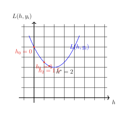
The graph above shows:
The loss function L(h, y_i) = \frac{1}{2}(h - 2)^2 + 3 as a blue curve.
The initial point h_0 = 0, the first update h_1 = 1, and the second update h_2 = 1.5 marked as red points.
The optimal height h^\ast = 2 shown as a dashed vertical line.
Determine whether the gradient descent algorithm will converge to the minimum of the loss function L(h, y_i). Explain your reasoning.
2in The loss function L(h, y_i) = \frac{1}{2}(h - y_i)^2 + 3 is a convex function because it is a quadratic function of h with a positive second derivative: \frac{\partial^2 L}{\partial h^2} = 1 > 0
Gradient descent will converge to the minimum of a convex function if the learning rate \eta is small enough, which is the case here.
[(12 points)] A sample space S is partitioned by three disjoint non-empty events E_1 \cup E_2 \cup E_3=S. Let A \subset S be an event and assume you are given the following probabilities: P(E_1),\hspace{.1in}P(E_2),\hspace{.1in}P(A \vert E_2),\hspace{.1in}P(A \vert E_3),\hspace{.1in}\text{ and }P(A \cap E_1). \bar{A} denotes the complement of A.
Show that the probability P(E_1 \vert \bar{A}) can be calculated using the above terms (i.e., no probability terms are missing in order to make this calculation).
True. P(E_1 \vert \bar{A}) = \frac{P(\bar{A} \cap E_1)}{P(\bar{A})} For the numerator P(\bar{A} \cap E_1) = P(\bar{A} \vert E_1) * P( E_1) which we can calculate as P(\bar{A} \vert E_1) = 1-P(A \vert E_1) P(A \vert E_1) = \frac{P(A \cap E_1)}{P(E_1)} Therefore P(\bar{A} \cap E_1) = P(E_1)-P(A \cap E_1). For the denominator we use the complement P(\bar{A}) = 1-P(A)
Using the law of total probability: P(A) = P(A \vert E_1) P(E_1) + P(A \vert E_2) P(E_2) + P(A \vert E_3) P(E_3) which we can calculate using P(E_3)=1-P(E_2)-P(E_1)
For parts (b), (c), and (d), you do not need to show your work for full credit, but partial credit may be awarded for supporting calculations and reasoning.
For the following statements, circle either TRUE or FALSE to indicate whether the equation is correct.
(i) P(\bar{E_1} \vert A) = P(E_2 \vert A) + P(E_3 \vert A)
| \bigcirc TRUE | \bigcirc FALSE |
(ii) P(\bar{A} \vert E_1) = 1 - P(\bar{E}_1 \vert \bar{A})
| \bigcirc TRUE | \bigcirc FALSE |
(iii) P(\bar{E_1} \vert A) = 1 - P(\bar{E}_1 \vert \bar{A})
| \bigcirc TRUE | \bigcirc FALSE |
Which of the following statements concerning E_1,E_2,E_3 are true? Only one statement is true.
| \bigcirc P(\overline{E_1} \cap \overline{E_2}) = 0 | \bigcirc P(\overline{E_1} \cup \overline{E_2}) \neq 0 |
| \bigcirc E1, E_2 and E_3 are independent events | \bigcirc P(E_1 \cup E_3) = 1 |
Correct: \overline{E_1} \cup \overline{E_2} = (E_2 \cup E_3) \cup (E_1 \cup E_3) = S \rightarrow P(\overline{E_1} \cup \overline{E_2}) = 1.
Incorrect: P(\overline{E_1} \cap \overline{E_2}) = P((E_2 \cup E3) \cap (E_1 \cup E_3)) = P(E_3) \neq 0
Incorrect: P(E_1 \cup E_3) = 1 - P(E_2) < 1 since E_2 is non empty.
Incorrect E1, E_2 and E_3 are not independent since P(E_1,E_2,E_3) = P(E_1 \cap E_2 \cap E_3) = P(\emptyset)= 0 \neq P(E_1)P(E_2)P(E_3)>0
If the event E_1 is fully contained within event A, i.e., every outcome in E_1 is also an outcome in A, we write that E_1 \subseteq A. Which if the following statements is true? Only one statement is true.
| \bigcirc If E_1 \subseteq A, then P(E_1)\leq P(A). |
| \bigcirc If P(E_1)\leq P(A), then E_1 \subseteq A. |
| \bigcirc If E_1 \subseteq A, then P(E_1 \cap A)\leq P(E_2). |
| \bigcirc If E_1 \subseteq A, then E_1 and A are independent events. |
| \bigcirc If E_1 \subseteq A, then E_3 and A are independent events. |
Correct: P(E_1) = \sum_{s \in E_1} p(s) and P(A) = \sum_{s \in A} p(s). Since \forall s \in E_1: s \in A, then P(E_1)\leq P(A).
The converse is not true: P(E_1)\leq P(A) can be true without E_1 \subseteq A.
When E_1 \subseteq A then P(E_1)=P(E_1 \cap A) however we don’t know anything about the relationship between P(E_1) and P(E_2).
If E_1 \subseteq A these are not independent events since P(E_1 | A) = 1 \neq P(E_1).
[(13 points)]
Robert has a sock drawer containing exactly eight socks: one pair each of plain socks, dotted socks, striped socks, and plaid socks.
On Monday morning while getting ready, Robert selects two socks at random from the drawer. What is the probability that the socks are matching? Explain your reasoning.
1in There are {8\choose 2} ways to pick the two socks from the drawer, of which exactly four pairs are matching. Therefore the probability is \frac{4}{{8\choose 2}} = \frac{(4)(2)}{(8)(7)} = \frac{1}{7}.
After wearing the socks on Monday he places them in a laundry basket separate from the drawer. On Tuesday morning, as Robert gets ready, he selects another two socks at random from the six remaining in the drawer. What is the probability that the socks are matching on Tuesday? Show all your calculations.
We can condition on whether the socks were matching on Monday and use this information to our advantage. Specifically,
\begin{align*} P[\text{match on Tues.}] &= P[\text{match on Tues.}|\text{match on Mon.}]P[\text{match on Mon.}] \\ &+ P[\text{match on Tues.}|\text{don't match on Mon.}]P[\text{don't match on Mon.}] \\ &= P[\text{match on Tues.}|\text{match on Mon.}]\frac{1}{7} \\ &+ P[\text{match on Tues.}|\text{don't match on Mon.}]\left(1 - \frac{1}{7}\right) \end{align*}
If the socks were matching on Monday, there are now three pairs of matching socks in the drawer. So we have, by the same logic as before,
\begin{align*} P[\text{match on Tues.}|\text{match on Mon.}] &= \frac{3}{\binom{6}{2}} = \frac{(3)(2)}{(6)(5)} = \frac{1}{5}. \end{align*}
If the socks were not matching on Monday, there are now two pairs of matching socks plus two mismatching socks. The total number of pairs is still \binom{6}{2} but now only two such pairs match. Therefore,
\begin{align*} P[\text{match on Tues.}|\text{don't match on Mon.}] &= \frac{2}{\binom{6}{2}} = \frac{(2)(2)}{(6)(5)} = \frac{2}{15}. \end{align*}
Thus in conclusion we have
\begin{align*} P[\text{match on Tues.}] &= \frac{1}{5}\cdot\frac{1}{7} + \frac{2}{15}\cdot\frac{6}{7}. \end{align*}
(\times6) On Tuesday evening Robert does laundry so that when he gets ready on Wednesday morning all of the socks are clean again. As usual he selects another two socks at random, a selection which is independent of any of his choices on Monday or Tuesday. What is the probability that he wears at least one striped sock on Monday, Tuesday, and Wednesday? Show all your calculations.
Based on the setup, Robert must have worn exactly one striped sock on both Monday and Tuesday, and then wore either a single striped sock or a pair of striped socks on Wednesday. By the definition of conditional probability, we have
P(\text{1 striped on Mon.} \cap \text{1 striped on Tues.}) = P(\text{1 striped on Tues.} \mid \text{1 striped on Mon.}) \times P(\text{1 striped on Mon.})
For Monday, there are \binom{2}{1}\binom{6}{1} = 12 possible pairs of socks so that exactly one is striped. Thus the probability is given by
P(\text{1 striped Mon.}) = \frac{12}{\binom{8}{2}} = \frac{(12)(2)}{(8)(7)} = \frac{3}{7}.
Alternatively, you could write this as 1 minus the probability of getting either no striped socks or two striped socks. For the second part, by similar logic, we have
P(\text{1 striped on Tues.} \mid \text{1 striped on Mon.}) = \frac{\binom{1}{1}\binom{5}{1}}{\binom{6}{2}} = \frac{(5)(2)}{(6)(5)} = \frac{1}{3}.
Therefore we have
P(\text{1 striped on Mon.} \cap \text{1 striped on Tues.}) = \frac{3}{7} \cdot \frac{1}{3} = \frac{1}{7}.
For Wednesday, he can select either one or two striped socks. Earlier we counted 12 pairs which contain exactly one striped sock, so there are 13 which contain either one or two. Thus
P(\text{1 or 2 striped on Weds.}) = \frac{13}{\binom{8}{2}} = \frac{13}{28}.
By the independence assumption, we have
\begin{align} &P(\text{1 striped on Mon.} \cap \text{1 striped on Tues.} \cap \geq\text{1 striped Weds.}) \\ &= P(\text{1 striped on Mon.} \cap \text{1 striped on Tues.}) \times P(\geq\text{1 striped Weds.}) \\ &= \frac{13}{(7)(28)} \end{align}
[(11 points)]
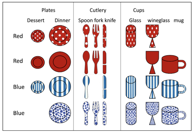
You have 4 sets of dishes each consisting of plates (dessert and dinner), cutlery (spoon fork and knife) and cups (glass, wineglass and mug). Two sets are red and two are blue and each set has a different pattern: dots, solid, stripes or flowers as in the picture below. Originally you had 4 * 8 =32 dishes, but over the years you have lost some of your dishes so that now you only have 28. A lost dish is indicated by dish being missing in the image (for example you lost the blue flowers dessert place or the red dots mug).
You come home and find a single item in the kitchen sick.
Let A be the event that the item has stripes, and let B be the event that the item is a cup (glass, wineglass or mug). Are these events independent? Explain your reasoning.
This question is based on the deck of cards question we did in class.
No, they are not. Knowing that the item is a cup makes it slightly more likely that the item has stripes.
P(A)=7/28 P(B)=10/28 = 5/14 P(A \cap B = 3/28 \neq (7*5)/(28*14)=5/56 Therefore not independent
Note this question is based on Lecture 23, slides 15, 20, 21 where we have replaced a deck of cards with patterned dishes.
In both b) and c) many made the mistake of selecting disjoint events A and B such the A \cap B = \emptyset (or A \cap B|C = \emptyset in c) ) but P(A),P(B)>0. Mutually exclusive events with non-zero probability are not independent (lecture 23, slide 13).
Regarding the identity of the item in the sink, give an example of two events A and B which are independent. Prove that they are independent. To receive full credit, your events should not have probabilities equal to zero or to one.
There were multiple correct options here.
One strategy is based on noticing that in every row there are 7 dishes. Therefore for any dish for which we have all 4 patterns (dinner plate, spoon, knife, wine glass) you can select event A to be a pattern (for example dots) and B to be one of the dishes for which we have the full set (for example spoon). Then P(A) = \frac{7}{28}=\frac{1}{4} P(B) = \frac{4}{28}=\frac{1}{7} P(A \cap B) = \frac{1}{28} = \frac{1}{7} \cdot \frac{1}{4}
Also P(B|A) = \frac{1}{7}=P(B)
This can also be done for either the red or blue color (instead of a single pattern), for example: Let A be the event that the item is red and let B be the event that the item is a spoon. There are 14 red dishes: P(A)=\frac{14}{28}=\frac{1}{2} and there are 4 spoons: P(B)=\frac{4}{28}=\frac{1}{7}. There are 2 red spoons: P(A,B) =\frac{2}{28}=\frac{1}{14}. P(A,B)= \frac{1}{14} =\frac{1}{7}* \frac{1}{2} =P(B)*P(A)
Regarding the identity of the item in the sink, give an example of three events A, B, and C such that A and B are conditionally independent given C. Prove that they are conditionally independent. To receive full credit, your events should not have probabilities equal to zero or to one.
As in b) there are many correct solutions here (some of you were very creative).
One strategy here is to consider the events in a) which weren’t independent and see if we can condition it on event C, so that they are. Let A be the event that the item has stripes, and let B be the event that the item is a cup (glass, wineglass or mug). Notice if we set C to be the event that the item is blue, none of the blue cups are missing.
Then, there are 3 blue striped cups: P(A\cap B|C)= \frac{3}{14}. There are seven blue striped dishes P(A|C)=\frac{7}{14}=\frac{1}{2} and there are 6 blue cups: P(B|C)=\frac{6}{14}=\frac{3}{7}. P(A\cap B|C)= \frac{3}{14} =\frac{1}{2}*\frac{3}{7}=P(A|C)*P(B|C)
Some other popular answers:
A = dots, B = plates, C= red (this also works for A = solid)
P(A|C) = \frac{7}{14}=\frac{1}{2} P(B|C) = \frac{4}{14}=\frac{2}{7} P(A \cap B|C) = \frac{2}{14}
A = stripe, B = knife, C= blue (this also works for A = flowers, and/or B = spoon) P(A|C) = \frac{7}{14}=\frac{1}{2} P(B|C) = \frac{2}{14}=\frac{1}{7} P(A \cap B|C) = \frac{1}{14}
We did accept cases (with some deduction) where P(A |C) =0 P(B|C)>0 P(A \cap B |C) =0
or P(A |C) =1 P(B|C)>0 P(A \cap B |C) = P(B|C)
[(8 points)] You work for Amazon and are implementing a book genre classifier to determine whether a book is science fiction (sci-fi), romance or thriller based on details of the plot. You have a dataset of 18 books and 4 features {“Happy conclusion",”Spaceships",“Murder investigation",”Sidekick" } to train a Naïve Bayes classifier.
| Book # | Genre | Murder | Sidekick | Happy | Spaceships |
| 1 | sci-fi | No | Yes | Yes | Yes |
| 2 | sci-fi | No | Yes | Yes | No |
| 3 | sci-fi | No | No | Yes | Yes |
| 4 | sci-fi | No | Yes | No | Yes |
| 5 | sci-fi | Yes | Yes | No | Yes |
| 6 | sci-fi | No | Yes | Yes | Yes |
| 7 | sci-fi | No | Yes | Yes | Yes |
| 8 | sci-fi | No | No | No | Yes |
| 9 | sci-fi | No | Yes | No | Yes |
| 10 | sci-fi | Yes | Yes | No | Yes |
| 11 | romance | No | No | Yes | Yes |
| 12 | romance | No | Yes | Yes | No |
| 13 | romance | No | Yes | Yes | No |
| 14 | romance | Yes | No | Yes | No |
| 15 | romance | No | No | Yes | No |
| 16 | romance | Yes | Yes | Yes | No |
| 17 | thriller | Yes | Yes | No | No |
| 18 | thriller | Yes | No | Yes | No |
| 19 | thriller | Yes | Yes | No | Yes |
| 20 | thriller | Yes | Yes | Yes | No |
(\times8) A new book has been released which has ’Happy conclusion", “sidekick" but not”Spaceships" or “murder investigation". Is this book a sci-fi, thriller or romance? Use the Naive Bayes Classifier without smoothing. Be sure to clearly state your prediction as one of the three genres. Show all your calculations.
We estimate the following probabilities from the table:
\begin{aligned} P(\text{Happy} \,|\,\text{romance}) & = 6/6=1 \\ P(\text{sidekick} \,|\,\text{romance}) & = 3/6=1/2 \\ P(\text{No Murder} \,|\,\text{romance}) & = 4/6=2/3 \\ P(\text{No Spaceships} \,|\,\text{romance}) & = 5/6 \\ P(\text{romance}) & = 6/20=3/10 \\[1em] P(\text{Happy} \,|\,\text{sci-fi}) & = 5/10 \\ P(\text{sidekick} \,|\,\text{sci-fi}) & = 8/10=4/5 \\ P(\text{No Murder} \,|\,\text{sci-fi}) & = 8/10=4/5 \\ P(\text{No Spaceships} \,|\,\text{sci-fi}) & = 1/10 \\ P(\text{sci-fi}) & = 10/20=1/2 \\[1em] P(\text{No Murder} \,|\,\text{thriller}) & = 0/4 \end{aligned}
\begin{aligned} & P(\text{romance} \mid \text{Happy,Sidekick, No Murder, No Spaceships}) \\ & \qquad \propto P(\text{Happy}\mid\text{romance}) \times P(\text{sidekick}\mid\text{romance}) \\ & \qquad \qquad \times P(\text{No Murder}\mid\text{romance}) \times P(\text{No Spaceships}\mid\text{romance}) \times P(\text{romance}) \\ & \qquad = 1 \cdot \frac{1}{2} \cdot \frac{2}{3} \cdot \frac{5}{6} \cdot \frac{3}{10} = \frac{1}{2} \cdot \frac{1}{3} \cdot \frac{1}{2} = \frac{1}{12} \end{aligned}
\begin{aligned} & P(\text{sci-fi} \mid \text{Happy,Sidekick, No Murder, No Spaceships}) \\ & \qquad \propto P(\text{Happy}\mid\text{sci-fi}) \times P(\text{sidekick}\mid\text{sci-fi}) \\ & \qquad \qquad \times P(\text{No Murder}\mid\text{sci-fi}) \times P(\text{No Spaceships}\mid\text{sci-fi}) \times P(\text{sci-fi}) \\ & \qquad = \frac{5}{10} \cdot \frac{4}{5} \cdot \frac{4}{5} \cdot \frac{1}{10} \cdot \frac{1}{2} = \frac{4}{5} \cdot \frac{1}{5} \cdot \frac{1}{10} = \frac{2}{125} \end{aligned}
\begin{aligned} & P(\text{thriller} \mid \text{Happy,Sidekick, No Murder, No Spaceships}) \\ & \qquad \propto P(\text{Happy}\mid\text{thriller}) \times P(\text{sidekick}\mid\text{thriller}) \\ & \qquad \qquad \times P(\text{No Murder}\mid\text{thriller}) \times P(\text{No Spaceships}\mid\text{thriller}) \times P(\text{thriller}) \\ & \qquad = 0 \end{aligned}
Since the first probability is the largest, our prediction is that the book was romance.